A few examples help build intuition for what the eigenvalues of the graph Laplacian tell us about a graph. The smallest eigenvalue is always zero (see explanation in footnote here).
For a complete graph on n vertices, all the eigenvalues except the first equal n. The eigenvalues of the Laplacian of a graph with n vertices are always less than or equal to n, this says the complete graph has the largest possible eigenvalue. This makes sense in light of the previous post: adding edges increases the eigenvalues. When you add as many edges as possible, you get the largest possible eigenvalues.
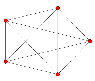
![\left[ \begin{array}{rrrrr} 4 & -1 & -1 & -1 & -1 \\ -1 & 4 & -1 & -1 & -1 \\ -1 & -1 & 4 & -1 & -1 \\ -1 & -1 & -1 & 4 & -1 \\ -1 & -1 & -1 & -1 & 4 \end{array} \right]](http://www.johndcook.com/complete_graph_laplacian.png)
Conversely, if all the non-zero eigenvalues of the graph Laplacian are equal, the graph is complete.
Next we look at the case of a star with n − 1 vertices connected to a central vertex. The smallest eigenvalue is zero, as always, and the largest is n. The ones in the middle are all 1. In particular, the second eigenvalue, the algebraic connectivity, is 1. It’s positive because the graph is connected, but it’s not large because the graph is not well connected: if you remove the central vertex it becomes completely disconnected.
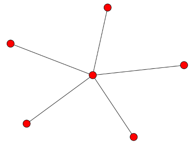
![\left[ \begin{array}{cccccc} 5 & -1 & -1 & -1 & -1 & -1 \\ -1 & 1 & 0 & 0 & 0 & 0 \\ -1 & 0 & 1 & 0 & 0 & 0 \\ -1 & 0 & 0 & 1 & 0 & 0 \\ -1 & 0 & 0 & 0 & 1 & 0 \\ -1 & 0 & 0 & 0 & 0 & 1 \end{array} \right]](http://www.johndcook.com/star_graph_laplacian.png)
Finally, we look at a cyclical graph, a ring with n vertices. Here the eigenvalues are 2 − 2 cos(2πk/n) where 0 ≤ k ≤ n/2. In particular, smallest non-zero eigenvalue is 2 − 2 cos(2π/n) and so as n increases, the algebraic connectivity approaches zero. This is curious since the topology doesn’t change at all. But from a graph theory perspective, a big ring is less connected than a small ring. In a big ring, each vertex is connected to a small proportion of the vertices, and the average distance between vertices is larger.
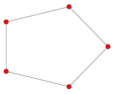
![\left[ \begin{array}{rrrrr} 2 & -1 & 0 & 0 & -1 \\ -1 & 2 & -1 & 0 & 0 \\ 0 & -1 & 2 & -1 & 0 \\ 0 & 0 & -1 & 2 & -1 \\ -1 & 0 & 0 & -1 & 2 \\ \end{array} \right]](http://www.johndcook.com/cycle_graph_laplacian.png)

