Imagine the following dialog.

Professor: f is a function of a real variable x that takes a real parameter k.

Student: What’s a parameter?

Professor: It’s a constant that can vary.

Student: Then if it can vary, isn’t it a variable?

Professor: Sorta, but no not really.

This conversation plays out over and over, and unfortunately it often ends as it does above, with the student confused. Here’s how I believe the conversation should continue.

Professor: You’re absolutely right that f is a function of two variables, x and k. But usually k is fixed in the context of a specific application and x is not. A different application might have a different, but also fixed, value of k. So it is helpful to think of f(x; k), a function of x with a parameter k, rather than f(x, k), a function of two variables. The former carries more information, giving a hint as to how the numbers are used.

Is there really a difference between a parameter and a variable? In a reductionistic sense, no. But in a practical sense, yes, absolutely.

It might sound pedantic to distinguish a variable from a parameter, and it is, in the best sense of the word. Pedant literally means teacher. Usually pedantic carries a negative connotation, such as making a distinction without a difference. But here the pedant would be making a helpful distinction.

For example, we might write a probability density function as f(x; μ, σ). The function gives the probability density at a point x. The density depends on parameters μ and σ, and these parameters change between applications, but for a given application they have fixed values.

You find the probability of a random variable taking on values in an interval [a, b] by integrating f over that interval. When I say that, you know that I mean you’d integrate with respect to x, because f is a function of x. It is also, in an abstract sense, a function of μ and σ, but it’s typically not useful to think of it that way.

Hypergeometric functions have two sets of parameters, and so you may see two semicolons, such as f(x; a, b; c). This denotes a function of the variable x, with upper parameters a and b, and a lower parameter c. In some abstract sense this is a function of four variables, but it acts very differently with respect to x than with respect to a, b, and c. There’s also a difference between a and b on the one hand and c on the other, one worth paying attention to, though it is less of a difference than between x and the parameters collectively.

Sometimes you’ll see a vertical bar rather than a semicolon to separate variables from parameters. This works out even better for probability densities because then f(x | μ, σ) suggests the probability density of x given μ and σ since the vertical bar is also used for conditional probability. You might also see f(x | a, b; c) for hypergeometric functions, with the vertical bar separating variables from parameters and the semicolon separating two kinds of parameters.

When I first saw a semicolon separating variables from parameters, no explanation was given, and I figured I could mentally replace the semicolon with a comma. Then later I realized that the semicolon was an act of kindness by the author giving the reader additional information.

Actuarial mathematics makes frequent use of a notation that as far as I know isn’t used anywhere else, and that is a bracket enclosing the northeast corner of a symbol.

This is used as subscript of another symbol, such as an a or an s, and there may be other decorations such more superscripts or subscripts.

For typesetting in LaTeX, the bracket is the only part that’s not standard. If you can put a bracket around a symbol, you can make the bracketed symbol a subscript just as you’d make anything else a subscript. LaTeX package actuarialangle lets you do this.

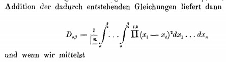
The angle notation that actuaries use for annuity-related calculations is not used anywhere else that I know of, but a variation was once used for factorials back in the 1800s, putting a bracket around the southwest corner of a symbol rather than the northeast. You can see examples here, including one use by David Hilbert.

Related post: Floor, ceiling, bracket

As longtime readers of this blog have probably noticed, I like to poke around in Unicode occasionally. It’s an endless system of rabbit holes to explore.

This morning I was looking at the Miscellaneous Mathematical Symbols block. These are mostly obscure symbols, though I’m sure for each symbol that I think is obscure, there is someone out there who uses it routinely.

Perpendicular

The only common symbol in this block is ⟂ (U+27C2) for perpendicular. Even so, this symbol is a variation on ⊥ (U+22A5). The distinction is semantic rather than visual: U+22A5 is used for the Boolean value “false.”

In addition to using ⟂ to denote perpendicular lines, some (e.g. Donald Knuth) use the symbol to denote that two integers are relatively prime.

Geometric algebra

The block contains ⟑ (U+27D1) which is used in geometric algebra for the geometric product, a.k.a. the dot-wedge product. The block also contains the symbol for the dual operator ⟇ (U+27c7), the geometric antiproduct. Incidentally, Eric Lengyel’s Projective Geometric Algebra site officially sponsors these two Unicode symbols.

I’m sure these symbols predate Eric Lengyel’s use of them, but I can only recall seeing them used in his work.

Database joins

Unicode has four symbols for database joins. The bowtie symbol ⨝ (U+2A1D) is used for inner (natural) joins is in another block. The Miscellaneous Mathematical Symbols block has three other symbols for outer joins: left, right, and full. I posted a table of these on @CompSciFact this morning.

pic.twitter.com/XXerIn5wrf

— Computer Science (@CompSciFact) April 14, 2025

Angle brackets

The Miscellaneous Mathematical Symbols block also has angle brackets: ⟨ (U+27E8) and ⟩ (U+27E9). These correspond to \langle and \rangle in LaTeX. I’ve used the LaTeX commands, but I wasn’t sure whether I’d ever used the Unicode characters. I searched this blog and found that I did indeed use the characters in my post on the Gram matrix.

More posts on math notation

• Floor, ceiling, bracket
• Up arrow notation
• Activation functions and Iverson brackets

I was looking today at a cardboard box that had the “this way up” symbol on it and wondered whether there is a Unicode value for it.

Apparently not. But there is an ISO code for it: ISO 7000 symbol 0623. It’s an international standard symbol for indicating how to orient a package. The name says it all: this way up.

There is a similar symbol in math and computer science: ↑↑. This is so-called up-arrow notation, introduced by Donald Knuth in 1976 [1].

In Knuth’s notation, ↑ indicates exponentiation, i.e. repeated multiplication, and ↑↑ indicates repeated exponentiation. There’s a little ambiguity here: we have to clarify in what order we apply exponentiation. Knuth stipulated that ↑↑ is right-associative, i.e.

So, for example, 5 ↑↑ 3 equals 5¹²⁵, not 125⁵.

In general, n arrows means to repeatedly apply n − 1 arrows. If we use ↑ⁿ as a shortcut for writing n up arrows, then we can define ↑ⁿ recursively as meaning we apply ↑ⁿ⁻¹ n times.

What I find most interesting about Knuth’s notation is how rarely it is used. I don’t think it’s because anyone object’s to Knuth’s notation; it’s just that there isn’t much need for what the notation represents. It’s primary use may be theoretical computer science. There you sometimes want to construct functions that grow ridiculously fast, such as Ackermann’s function, and functions of the form a ↑ⁿ b are good for that.

This is curious. Multiplication is repeated addition, exponentiation is repeated multiplication, and so repeated exponentiation seems like a natural extension. I won’t say that it’s unnatural, but it is very uncommon.

Related posts

• Engine coolant temperature symbol
• Conditional independence notation
• i^i^i …

[1] Donald E. Knuth. “Mathematics and Computer Science: Coping with Finiteness”. Science. 194 (4271): 1235–1242.

The factorial of an integer n is the product of the positive integers up to n.

The double factorial of an even (odd) integer n is the product of the positive even (odd) integers up to n. For example,

8!! = 8 × 6 × 4 × 2

and

9!! = 9 × 7 × 5 × 3 × 1.

Double factorials come up fairly often, and sometimes triple, quadruple, or higher multifactorials do too.

In general, the k-factorial of n is the product of the positive integers up to n that are congruent to n mod k. Here’s how you might implement k-factorials in Python.

    from operator import mul
    from functools import reduce

    def multifactorial(n, k):
        return reduce(mul, [i for i in range(1, n+1) if (n-i)%k == 0], 1)

Update: As pointed out in the comments, multifactorial could be implemented more succinctly as

    def multifactorial(n, k):
        return reduce(mul, range(n, 0, -k), 1)

Factorial notation is a little awkward, and multifactorial notation is even more awkward. Someone seeing n!! for the first time might reasonably assume it means (n!)!, but it does not.

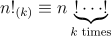
Adding exclamation points works, albeit awkwardly, for specific values of k, but not for variable numbers of k. One way I’ve seen to express k-factorials for variable k is to add a subscript (k) to the factorial:

I’ve also seen the subscript on the exclamation point written as a superscript instead.

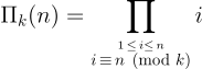
I’d like to suggest a different notation: Π_k. by analogy with the Π function.

When k ≡ 1 the condition i ≡ n (mod k) always holds, and we have factorial, i.e.

Π₁(n) = Π(n) = n!.

One downside of this notation is that while the function Π is defined for all complex numbers (aside from singularities at negative integers) the function Π_k is only defined for positive integer arguments. Still, in my opinion, this is less awkward than the alternatives I’ve seen.

By the way, the term “double factorial” seems backward. Maybe it should have been “half factorial” because you’re multiplying half as many numbers together, not twice as many. “Multifactorial” in general seems like an unfortunate name. Subfactorial might have been better, but unfortunately that name means something else.

I understand why someone may have come up with the idea of using two exclamation points for what we call double factorial; it would be hard to draw half an exclamation point. An advantage of the notation suggested here is that it suggests that there’s a variation on factorial somehow associated with k, but there’s no implication of multiplying or dividing by k.

Adding “mod k” as a subscript would be even more explicit than a subscript k. Someone who hadn’t seen

Π_{mod k} (n)

before might be able to figure out what it means; I think they would at least easily remember what it means once told. And the presence of “mod” might suggest to the reader that the argument needs to be an integer.

Mathematics notation changes slowly over time, generally for the better. I can’t think of an instance that I think was a step backward.

Gauss introduced the notation [x] for the greatest integer less than or equal to x in 1808. The notation was standard until relatively recently, though some authors used the same notation to mean the integer part of x. The two definitions agree if x is positive, but not if x is negative.

Not only is there an ambiguity between the two meanings of [x], it’s not immediately obvious that there is an ambiguity since we naturally think first of positive numbers. This leads to latent errors, such as software that works fine until the first person gives something a negative input.

In 1962 Kenneth Iverson introduced the notation ⌊x⌋ (“floor of x“) and ⌈x⌉ (“ceiling of x“) in his book A Programming Language, the book that introduced APL. According to Concrete Mathematics, Iverson

found that typesetters could handle the symbols by shaving off the tops and bottoms of ‘[‘ and ‘]’.

This slight modification of the existing notation made things much clearer. The notation [x] is not mnemonic, but clearly ⌊x⌋ means to move down and ⌈x⌉ means to move up.

Before Iverson introduced his ceiling function, there wasn’t a standard notation for the smallest integer greater than or equal to x. If you did need to refer to what we now call the ceiling function, it was awkward to do so. And if there was a symmetry in some operation between rounding down and rounding up, the symmetry was obscured by asymmetric notation.

My impression is that ⌊x⌋ became more common than [x] somewhere around 1990, maybe earlier in computer science and later in mathematics.

Iverson and APL

Iverson’s introduction of the floor and ceiling functions was brilliant. The notation is mnemonic, and it filled what in retrospect was a gaping hole. In hindsight, it’s obvious that if you have a notation for what we now call floor, you should also have a notation for what we now call ceiling.

Iverson also introduced the indicator function notation, putting a Boolean expression in brackets to denote the function that is 1 when the expression is true and 0 when the expression is false. Like his floor and ceiling notation, the indicator function notation is brilliant. I give an example of this notation in action here.

I had a small consulting project once where my main contribution was to introduce indicator function notation. That simple change in notation made it clear how to untangle a complicated calculation.

Since two of Iverson’s notations were so simple and useful, might there be more? He introduced a lot of new notations in his programming language APL, and so it makes sense to mine APL for more notations that might be useful. But at least in my experience, that hasn’t paid off.

I’ve tried to read Iverson’s lecture Notation as a Tool of Thought several times, and every time I’ve given up in frustration. Judging by which notations have been widely adopted, the consensus seems to be that the floor, ceiling, and indicator function notations were the only ones worth stealing from APL.

This evening I ran across a dialog that suggests that decimal notation is wrong.

It happened when I started learning about decimals in school. I knew then that ten has one zero, a hundred has two, a thousand three, and so on. And then this teacher starts saying that tenth doesn’t have any zero, a hundredth has only one, a thousandth has only two, and so on. … Only much later did I have enough perspective to put my finger on the problem: The decimal point is always misplaced!

Source: Conics. Emphasis in the original.

The proposed solution is to put the decimal point above the units position rather than after it. Then the notation would be symmetric. For example, 1000 and 1/1000 would look like this:

Of course decimal notation isn’t likely to change, but the author makes an interesting point.