The orbit that put men on the moon

Posted on 8 February 2020 by John

Richard Arenstorf (1929–2014) discovered a stable periodic orbit between the Earth and the Moon which was used as the basis for the Apollo missions.

His orbit is a special case of the three body problem where two bodies are orbiting in a plane, i.e. the Earth and the Moon, along with a third body of negligible mass relative to the other bodies, i.e. the satellite.

The system of differential equations for the Arenstorf orbit are

$\begin{align*} x'' &= x + 2y' - \mu' \frac{x+\mu}{D_1} - \mu \frac{x - \mu'}{D_2} \\ y'' &= y - 2x' - \mu' \,\frac{y}{\,D_1} \,\,\,\,\,\,- \mu \frac{y}{\,D_2} \\ \end{align*}$

where

$\begin{align*} D_1 &= ((x + \mu)^2 \,+ y^2)^{3/2} \\ D_2 &= ((x - \mu')^2 + y^2)^{3/2} \end{align*}$

Here the Earth is at the origin and the Moon is initially at (0, 1). The mass of the Moon is μ = 0.012277471 and the mass of the Earth is μ’ = 1 − μ.

The initial conditions are

$\begin{align*} x(0) &= \phantom{-}0.994 \\ x'(0) &= \phantom{-}0 \\ y(0) &= \phantom{-}0 \\ y'(0) &= -2.001585106 \end{align*}$

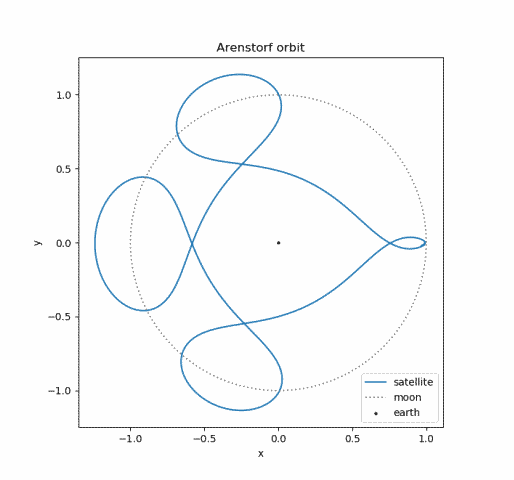
Here’s a plot of the orbit.

Arenstorf orbit

I found the equations above in [1] which sites the original paper [2]. Note that the paper was written in 1963, seven years before the Apollo missions. Also, before leaving NASA Arenstorf mapped out a rescue orbit. This orbit was later used on Apollo 13.

Richard Arenstorf

I was fortunate to do my postdoc at Vanderbilt before Arenstorf retired and was able to sit in on an introductory course he taught on orbital mechanics. His presentation was leisurely and remarkably clear.

His course was old-school “hard analysis,” much more concrete than the abstract “soft analysis” I had studied in graduate school. He struck me as a 19th century mathematician transported to the 20th century.

He scoffed at merely measurable functions. “Have you ever seen a function that wasn’t analytic?” This would have been heresy at my alma mater.

When I asked him about “Arenstorf’s theorem” from a recently published book I was reading, he said that he didn’t recognize it. I forget now how it was stated, maybe involving Banach spaces and/or manifolds. Arenstorf was much more concrete. He wanted to help put a man on the Moon, not see how abstractly he could state his results.

Orbital resonance in Neptune’s moons

Posted on 17 November 2019 by John

Phys.com published an article a couple days ago NASA finds Neptune moons locked in ‘dance of avoidance’. The article is based on the scholarly paper Orbits and resonances of the regular moons of Neptune.

The two moons closest to Neptune, named Naiad and Thalassa, orbit at nearly the same distance, 48,224 km for Naiad and 50,074 km for Thalassa. However, the moons don’t come as close to each other as you would expect from looking just at the radii of their orbits.

Although the radii of the orbits differ by 1850 km, the two moons do not get closer than about 2800 km apart. The reason has to do with the inclination of the two orbital planes with each other, and a resonance between their orbital periods. When the moons approach each other, one dips below the other, increasing their separation.

Assume the orbits of both moons are circular. (They very nearly are, with major and minor axes differing by less than a kilometer.) Also, choose a coordinate system so that Thalassa orbits in the xy plane. The position of Thalassa at time t is

r_T (cos 2πt/T_T, sin 2πt/T_T, 0)

where r_T is the radius of Thalassa’s orbit and T_T is its period.

The orbit of Naiad is inclined to that of Thalassa by an angle u. The position of Naiad at time t is

r_N (cos u cos 2πt/T_N, sin 2πt/T_N, -sin u cos 2πt/T_N).

I tried implementing the model above using data from Wikipedia articles on the two moons, but in my calculations the moons get closer than reported. I suspect the parameters have to be set carefully in order to demonstrate the kind of resonance we see in observation, and we don’t know these parameters accurately enough to make a direct geometric approach like this work.

from numpy import *

# Orbital radii in km 
r_T = 50074.44
r_N = 48224.41

# Period in days
T_T = 0.31148444
T_N = 0.29439580

def thalassa(t):

    # frequency
    f = 2*pi/T_T

    return r_T * array([
        cos(f*t),
        sin(f*t),
        0
    ])

def naiad(t):
    
    # inclination in radians relative to Thalassa
    i = 0.082205
    
    # frequency
    f = 2*pi/T_N

    return r_N * array([
        cos(i)*cos(f*t),
        sin(f*t),
        -sin(i)*cos(f*t)
    ])

def dist(t):
    return sum((naiad(t) - thalassa(t))**2)**0.5

d = [dist(t) for t in linspace(0, 10*73*T_N, 1000)]
print(d[0], min(d))

In this simulation, the moons are 4442 km apart when t = 0, but this is not the minimum distance. The code above shows an instance where the distance is 2021 km. I tried minor tweaks, such as adding a phase shift to one of the planets or varying the angle of inclination, but I didn’t stumble on anything that cane closer to reproducing the observational results. Maybe resonance depends on factors I’ve left out. Naiad and Thalassa are practically massless compared to Neptune, but perhaps the simulation needs to account for their mass.

The periods of the two moons are nearly in a ratio of 69 to 73. We could idealize the problem by making the periods rational numbers in exactly a ratio of 69 to 73. Then the system would be exactly periodic, and we could find the minimum distance. Studying a model system close to the real one might be useful. If we do tweak the periods, we’d need to tweak the radii as well so that Kepler’s third law applies, i.e. we’d need to keep the squares of the periods proportional to the cubes of the radii.

Related post: Average distance between planets

Kepler and the contraction mapping theorem

Posted on 21 December 2018 by John

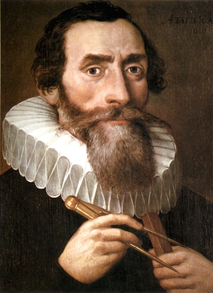
Johannes Kepler

The contraction mapping theorem says that if a function moves points closer together, then there must be some point the function doesn’t move. We’ll make this statement more precise and give a historically important application.

Definitions and theorem

A function f on a metric space X is a contraction if there exists a constant q with 0 ≤ q < 1 such that for any pair of points x and y in X,

d( f(x), f(y) ) ≤ q d(x, y)

where d is the metric on X.

A point x is a fixed point of a function f if f(x) = x.

Banach’s fixed point theorem, also known as the contraction mapping theorem, says that every contraction on a complete metric space has a fixed point. The proof is constructive: start with any point in the space and repeatedly apply the contraction. The sequence of iterates will converge to the fixed point.

Application: Kepler’s equation

Kepler’s equation in for an object in an elliptical orbit says

M + e sin E = E

where M is the mean anomaly, e is the eccentricity, and E is the eccentric anomaly. These “anomalies” are parameters that describe the location of an object in orbit. Kepler solved for E given M and e using the contraction mapping theorem, though he didn’t call it that.

Kepler speculated that it is not possible to solve for E in closed form—he was right—and used a couple iterations [1] of

f(E) = M + e sin E

to find an approximate fixed point. Since the mean anomaly is a good approximation for the eccentric anomaly, M makes a good starting point for the iteration. The iteration will converge from any starting point, as we will show below, but you’ll get a useful answer sooner starting from a good approximation.

Proof of convergence

Kepler came up with his idea for finding E around 1620, and Banach stated his fixed point theorem three centuries later. Kepler had the idea of Banach’s theorem, but he didn’t have a rigorous formulation of the theorem or a proof.

In modern terminology, the real line is a complete metric space and so we only need to prove that the function f above is a contraction. By the mean value theorem, it suffices to show that the absolute value of its derivative is less than 1. That is, we can use an upper bound on |f ‘| as the q in the definition of contraction.

Now

f ‘ (E) = e cos E

and so

|f ‘(E)| ≤ e

for all E. If our object is in an elliptical orbit, e < 1 and so we have a contraction.

Example

The following example comes from [2], though the author uses Newton’s method to solve Kepler’s equation. This is more efficient, but anachronistic.

Consider a satellite on a geocentric orbit with eccentricity e = 0.37255. Determine the true anomaly at three hours after perigee passage, and calculate the position of the satellite.

The author determines that M = 3.6029 and solves Kepler’s equation

M + e sin E = E

for E, which she then uses to solve for the true anomaly and position of the satellite.

The following Python code shows the results of the first 10 iterations of Kepler’s equation.

    from math import sin

    M = 3.6029
    e = 0.37255

    E = M
    for _ in range(10):
        E = M + e*sin(E)
        print(E)

This produces

and so it appears the iteration has converged to E = 3.4794 to four decimal places.

Note that this example has a fairly large eccentricity. Presumably Kepler would have been concerned with much smaller eccentricities. The eccentricity of Jupiter’s orbit, for example, is around 0.05. For such small values of e the iteration would converge more quickly.

Update: See this post for more efficient ways to solve Kepler’s equation.

[1] Bertil Gustafsson saying in his book Scientific Computing: A Historical Perspective that Kepler only used two iterations. Since M gives a good starting approximation to E, two iterations would give a good answer. I imagine Kepler would have done more iterations if necessary but found empirically that two was enough. Incidentally, it appears Gustaffson has a sign error in his statement of Kepler’s equation.

[2] Euler Celestial Analysis by Dora Musielak.

Orbital mechanics