I never heard of Bessel or Everett interpolation until long after college. I saw Lagrange interpolation several times. Why Lagrange and not Bessel or Everett?
First of all, Bessel interpolation and Everett interpolation are not different kinds of interpolation; they are different algorithms for carrying out the same interpolation as Lagrange. There is a unique polynomial of degree n fitting a function at n + 1 points, and all three methods evaluate this same polynomial.
The advantages of Bessel’s approach or Everett’s approach to interpolation are practical, not theoretical. In particular, these algorithms are practical when interpolating functions from tables, by hand. This was a lost art by the time I went to college. Presumably some of the older faculty had spent hours computing with tables, but they never said anything about it.
Bessel interpolation and Everett interpolation are minor variations on the same theme. This post will describe both at such a high level that there’s no difference between them. This post is high-level because that’s exactly what seems to be missing in the literature. You can easily find older books that go into great detail, but I believe you’ll have a harder time finding a survey presentation like this.
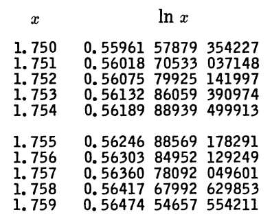
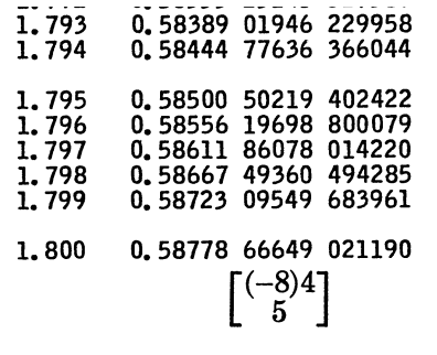
Suppose you have a function f(x) that you want to evaluate at some value p. Without loss of generality we can assume our function has been shifted and scaled so that we have tabulated f at integers our value p lies between 0 and 1.
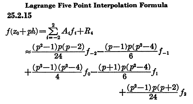
Everett’s formula (and Bessel’s) cleanly separates the parts of the interpolation formula that depend on f and the parts that depend on p.
The values of the function f enter through the differences of the values of f at consecutive integers, and differences of these differences, etc. These differences are easy to calculate by hand, and sometimes were provided by the table publisher.
The functions of p are independent of the function being interpolated, so these functions, the coefficients in Bessel’s formula and Everett’s formula, could be tabulated as well.
If the function differences are tabulated, and the functions that depend on p are tabulated, you could apply polynomial interpolation without ever having to explicitly evaluate a polynomial. You’d just need to evaluate a sort of dot product, a sum of numbers that depend on f multiplied by numbers that depend on p.
Another advantage of Bessel’s and Everett’s interpolation formulas is that they can be seen as a sequence of refinements. First you obtain the linear interpolation result, then refine it to get the quadratic interpolation result, then add terms to get the cubic interpolation result, etc.
This has several advantages. First, you have the satisfaction of seeing progress along the way; Lagrange interpolation may give you nothing useful until you’re done. Related to this is a kind of error checking: you have a sense of where the calculations are going, and intermediate results that violate your expectations are likely to be errors. Finally, you can carry out the calculations for the smallest terms in with less precision. You can use fewer and fewer digits in your hand calculations as you compute successive refinements to your result.