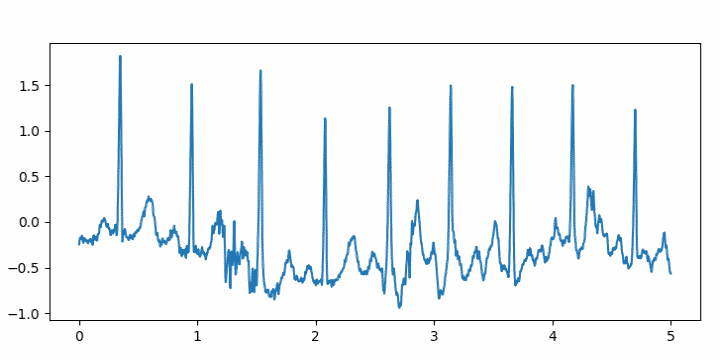
I was browsing through SciPy documentation this evening and ran across a function in scipy.misc called electrocardiogram. What?!
It’s an actual electrocardiogram, sampled at 360 Hz. Presumably it’s included as convenient example data. Here’s a plot of the first five seconds.
I wrote a little code using it to turn the ECG into an audio file.
from numpy import int16, iinfo
from scipy.io.wavfile import write
from scipy.misc import electrocardiogram

def to_integer(signal):
    # Take samples in [-1, 1] then scale to 16-bit integers
    m = iinfo(int16).max
    M = max(abs(signal))
    return int16(signal*m/M)

ecg = electrocardiogram()
write("heartbeat.wav", 360, to_integer(ecg))
I had to turn the volume way up to hear it, and that made me think of Edgar Allan Poe’s story The Tell-Tale Heart.
I may be doing something wrong. According to the documentation for the write function, I shouldn’t need to convert the signal to integers. I should just be able to leave the signal as floating point and normalize it to [−1, 1] by dividing by the largest absolute value in the signal. But when I do that, the output file will not play.
I’ve made a couple minor changes to my page that converts between frequency and pitch. (The page also includes Barks, a psychoacoustic unit of measure.)
If you convert a frequency in Hertz to musical notation, the page used to simply round to the nearest note in the chromatic scale. Now the page will also tell you how sharp or flat the pitch is if it’s not exact.
For example, if you enter 1100 Hz, the page used to report simply “C#6” and now it reports “C#6 − 14 cents” meaning the closest note is C#6, but it’s a little flat, 14/100 of a semitone flat. If you enter 1120 Hz it will report “C#6 + 18 cents” meaning that the note is 18/100 of a semitone sharp.
Octave numbers, such as the 6 in C#6 are explained here.
The other change I made to the page was to add a little eighth note favicon that might show up in a browser tab.
I’ve written several online converters like this: LaTeX to Unicode, wavelength to RGB, etc. See a full list here.
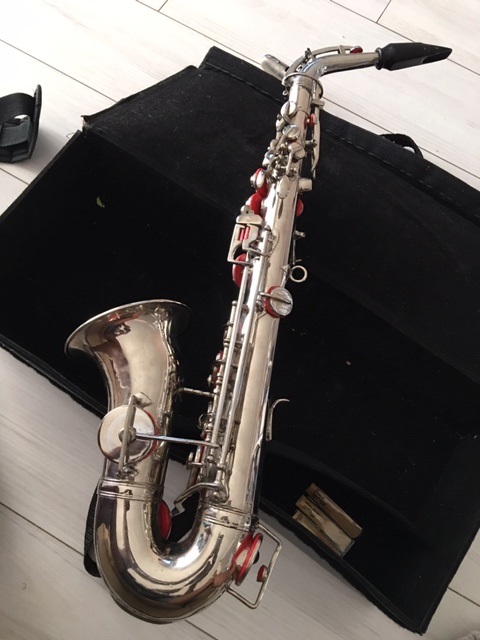
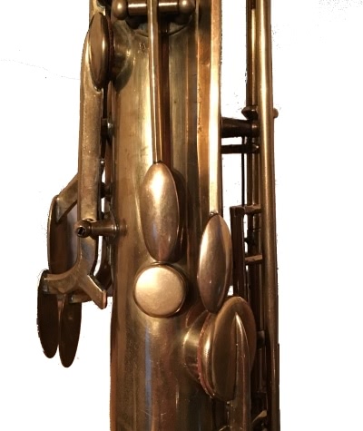
Paul A. sent me a photo of his alto sax in response to my previous post on a saxophone with two octave keys. His saxophone also has two octave keys, and it has a short bell. Contemporary saxophones have a longer bell, go down to B flat, and have two large pads on the bell. Paul’s saxophone has a shorter bell, only goes down to B, and only has one pad on the bell.
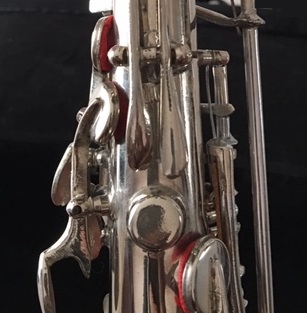
Here’s a closeup of the octave keys.
Paul says he found his instrument in an antique shop. It has no serial number or manufacturer information. If you know anything about this model, please leave a comment below.
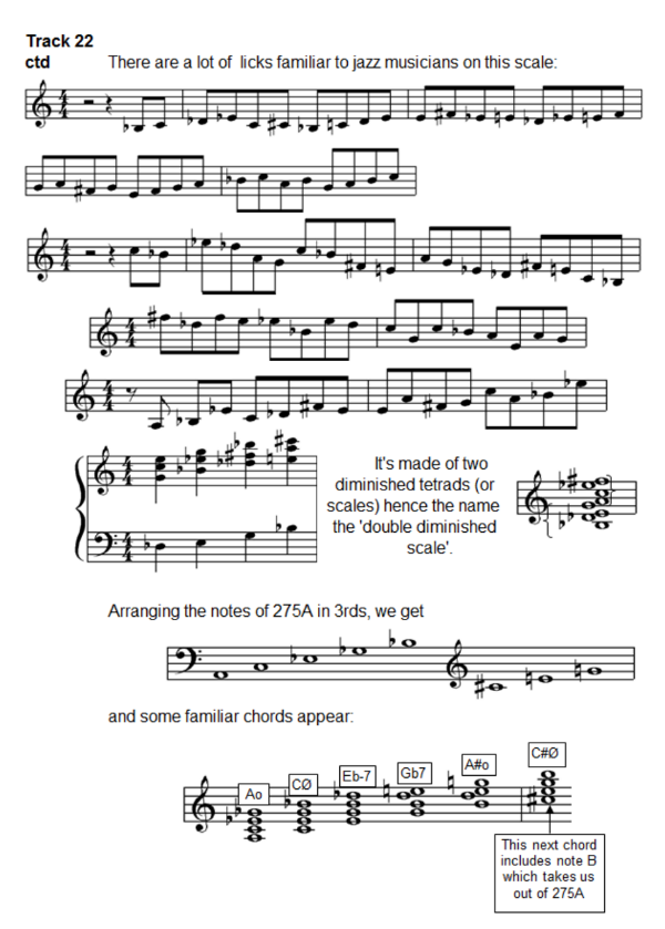
Pete White contacted me in response to a blog post I wrote enumerating musical scales. He has written a book on the subject, with audio, that he is giving away. He asked if I would host the content, and I am hosting it here.
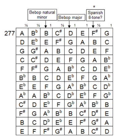
Here are a couple screen shots from the book to give you an idea what it contains.
Here’s an example scale, number 277 out of 344.
And here’s an example of the notes for the accompanying audio files.
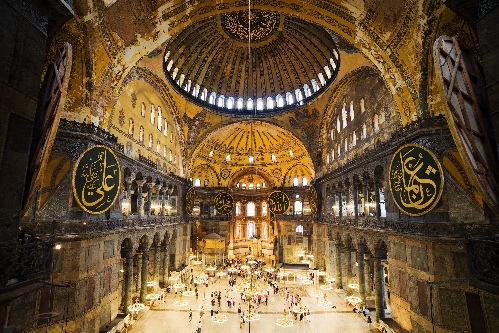
The Hagia Sophia (Greek for “Holy Wisdom”) was a Greek Orthodox cathedral from 537 to 1453. When the Ottoman Empire conquered Constantinople the church was converted into a mosque. Then in 1935 it was converted into a museum.
No musical performances are allowed in the Hagia Sophia. However, researchers from Stanford have modeled the acoustics of the space in order to simulate what worship would have sounded like when it was a medieval cathedral. The researchers recorded a virtual performance by synthesizing the acoustics of the building. Not only did they post-process the sound to give the singers the sound of being in the Hagia Sophia, they first gave the singers real-time feedback so they would sing as if they were there.
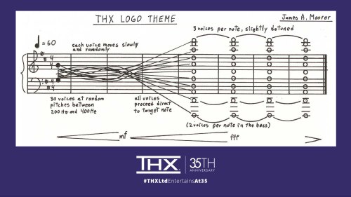
I just finished listening to the latest episode of Twenty Thousand Hertz, the story behind “Deep Note,” the THX logo sound.
There are a couple mathematical details of the sound that I’d like to explore here: random number generation, and especially Pythagorean tuning.
Random number generation
First is that part of the construction of the sound depended on a random number generator. The voices start in a random configuration and slowly reach the target D major chord at the end.
Apparently the random number generator was not seeded in a reproducible way. This was only mentioned toward the end of the show, and a teaser implies that they’ll go more into this in the next episode.
Pythagorean tuning
The other thing to mention is that the final chord is based on Pythagorean tuning, not the more familiar equal temperament.
The lowest note in the final chord is D1. (Here’s an explanation of musical pitch notation.) The other notes are D2, A2, D3, A3, D4, A4, D5, A5, D6, and F#6.
Octaves
Octave frequencies are a ratio of 2:1, so if D1 is tuned to 36 Hz, then D2 is 72 Hz, D3 is 144 Hz, D4 is 288 Hz, D5 is 576 Hz, and D6 is 1152 Hz.
Fifths
In Pythagorean tuning, fifths are in a ratio of 3:2. In equal temperament, a fifth is a ratio of 27/12 or 1.4983 [1], a little less than 3/2. So Pythagorean fifths are slightly bigger than equal temperament fifths. (I explain all this here.)
If D2 is 72 Hz, then A2 is 108 Hz. It follows that A3 would be 216 Hz, A4 would be 432 Hz (flatter than the famous A 440), and A5 would be 864 Hz.
Major thirds
The F#6 on top is the most interesting note. Pythagorean tuning is based on fifths being a ratio of 3:2, so how do you get the major third interval for the highest note? By going up by fifths 4 times from D4, i.e. D4 -> A4 -> E5 -> B5 -> F#6.
The frequency of F#6 would be 81/16 of the frequency of D4, or 1458 Hz.
The F#6 on top has a frequency 81/64 that of the D# below it. A Pythagorean major third is a ratio of 81/64 = 1.2656, whereas an equal temperament major third is f 24/12 or 1.2599 [2]. Pythagorean tuning makes more of a difference to thirds than it does to fifths.
A Pythagorean major third is sharper than a major third in equal temperament. Some describe Pythagorean major chords as brighter or sweeter than equal temperament chords. That the effect the composer was going for and why he chose Pythagorean tuning.
Detuning
Then after specifying the exact pitches for each note, the composer actually changed the pitches of the highest voices a little to make the chord sound fuller. This makes the three voices on each of the highest notes sound like three voices, not just one voice. Also, the chord shimmers a little bit because the random effects from the beginning of Deep Note never completely stop, they are just diminished over time.
How many musical scales are there? That’s not a simple question. It depends on how you define “scale.”
For this post, I’ll only consider scales starting on C. That is, I’ll only consider changing the intervals between notes, not changing the starting note. Also, I’ll only consider subsets of the common chromatic scale; this post won’t get into dividing the octave into more or less than 12 intervals.
First of all we have the major scale — C D E F G A B C — and the “natural” minor scale: A B C D E F G A. The word “natural” suggests there are other minor scales. More on that later.
Then we have the classical modes: Dorian, Phrygian, Lydian, Mixolydian, Aeolian, and Locrian. These have the same intervals as taking the notes of the C major scale and starting on D, E, F, G, A, and B respectively. For example, Dorian has the same intervals as D E F G A B C D. Since we said we’d start everything on C, the Dorian mode would be C D E♭ F G A B♭ C. The Aeolian mode is the same as the natural minor scale.
The harmonic minor scale adds a new wrinkle: C D E♭ F G A♭ B C. Notice that A♭ and B are three half steps apart. In all the scales above, notes were either a half step or a whole step apart. Do we want to consider scales that have such large intervals? It seems desirable to include the harmonic minor scale. But what about this: C E♭ G♭ A C. Is that a scale? Most musicians would think of that as a chord or arpeggio rather than a scale. (It’s a diminished seventh chord. And it would be more common to write the A as a B♭♭.)
We might try to put some restriction on the definition of a scale so that the harmonic minor scale is included and the diminished seventh arpeggio is excluded. Here’s what I settled on. For the purposes of this post, I’ll say that a scale is an ascending sequence of eight notes with two restrictions: the first and last are an octave apart, and no two consecutive notes are more than three half steps apart. This will include modes mentioned above, and the harmonic minor scale, but will exclude the diminished seventh arpeggio. (It also excludes pentatonic scales, which we may or may not want to include.)
One way to enumerate all possible scales would be to start with the chromatic scale and decide which notes to keep. Write out the notes C, C♯, D, … , B, C and write a ‘1’ underneath a note if you want to keep it and a ‘0’ otherwise. We have to start and end on C, so we only need to specify which of the 11 notes in the middle we are keeping. That means we can describe any potential scale as an 11-bit binary number. That’s what I did to carry out an exhaustive search for scales with a little program.
There are 266 scales that meet the criteria listed here. I’ve listed all of them on another page. Some of these scales have names and some don’t. I’ve noted some names as shown below. I imagine there are others that have names that I have not labeled. I’d appreciate your help filling these in.
|--------------+-----------------------+-------------------|
| Scale number | Notes                 | Name              |
|--------------+-----------------------+-------------------|
|          693 | C D  E  F# G  A  B  C | Lydian mode       |
|          725 | C D  E  F  G  A  B  C | Major             |
|          726 | C D  E  F  G  A  Bb C | Mixolydian mode   |
|          825 | C D  Eb F# G  Ab B  C | Hungarian minor   |
|          826 | C D  Eb F# G  Ab Bb C | Ukrainian Dorian  |
|          854 | C D  Eb F  G  A  Bb C | Dorian mode       |
|          858 | C D  Eb F  G  Ab Bb C | Natural minor     |
|         1235 | C Db E  F  G  Ab B  C | Double harmonic   |
|         1242 | C Db E  F  G  Ab Bb C | Phrygian dominant |
|         1257 | C Db E  F  Gb Ab B  C | Persian           |
|         1370 | C Db Eb F  G  Ab Bb C | Phrygian mode     |
|         1386 | C Db Eb F  Gb Ab Bb C | Locrian mode      |
|--------------+-----------------------+-------------------|
Update: See this page for Pete White’s free ebook listing all possible scales with 3 to 11 notes.
Last year I wrote a post about saxophone octave keys. I was surprised to discover, after playing saxophone for most of my life, that a saxophone has not one but two octave holes. Modern saxophones have one octave key, but two octave holes. Originally saxophones had a separate octave key for each octave hole; you had to use different octave keys for different notes.
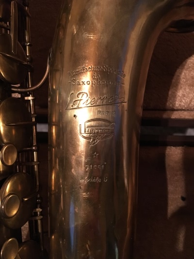
I had not seen one of these old saxophones until Carlo Burkhardt sent me photos today of a Pierret Modele 5 Tenor Sax from around 1912.
Here’s a closeup of the octave keys.
And here’s a closeup of the bell where you can see the branding.
Update (2019-01-22): A reader, Paul A., sent me photos of a silver alto sax with two octave keys. More on this saxophone here.
The other day I wrote about the golden angle, a variation on the golden ratio. If φ is the golden ratio, then a golden angle is 1/φ2 of a circle, approximately 137.5°, a little over a third of a circle.
Musical notes go around in a circle. After 12 half steps we’re back where we started. What would it sound like if we played intervals that went around this circle at golden angles? I’ll include audio files and the code that produced them below.
A golden interval, moving around the music circle by a golden angle, is a little more than a major third. And so a chord made of golden intervals is like an augmented major chord but stretched a bit.
An augmented major triad divides the musical circle exactly in thirds. For example, C E G#. Each note is four half steps, a major third, from the previous note. In terms of a circle, each interval is 120°. Here’s what these notes sound like in succession and as a chord.
If we go around the musical circle in golden angles, we get something like an augmented triad but with slightly bigger intervals. In terms of a circle, each note moves 137.5° from the previous note rather than 120°. Whereas an augmented triad goes around the musical circle at 0°, 120°, and 240° degrees, a golden triad goes around 0°, 137.5°, and 275°.
A half step corresponds to 30°, so a golden angle corresponds to a little more than 4.5 half steps. If we start on C, the next note is between E and F, and the next is just a little higher than A.
If we keep going up in golden intervals, we do not return to the note we stared on, unlike a progression of major thirds. In fact, we never get the same note twice because a golden interval is not a rational part of a circle. Four golden angle rotations amount to 412.5°, i.e. 52.5° more than a circle. In terms of music, going up four golden intervals puts us an octave and almost a whole step higher than we stared.
Here’s what a longer progression of golden intervals sounds like. Each note keeps going but decays so you can hear both the sequence of notes and how they sound in harmony. The intention was to create something like playing the notes on a piano with the sustain pedal down.
It sounds a little unusual but pleasant, better than I thought it would.
Here’s the Python code that produced the sound files in case you’d like to create your own. You might, for example, experiment by increasing or decreasing the decay rate. Or you might try using richer tones than just pure sine waves.
from scipy.constants import golden
import numpy as np
from scipy.io.wavfile import write

N = 44100 # samples per second

# Inputs:
# frequency in cycles per second
# duration in seconds
# decay = half-life in seconds
def tone(freq, duration, decay=0):
    t = np.arange(0, duration, 1.0/N)
    y = np.sin(freq*2*np.pi*t)
    if decay > 0:
        k = np.log(2) / decay
        y *= np.exp(-k*t)
    return y

# Scale signal to 16-bit integers,
# values between -2^15 and 2^15 - 1.
def to_integer(signal):
    signal /= max(abs(signal))
    return np.int16(signal*(2**15 - 1))

C = 262 # middle C frequency in Hz

# Play notes sequentially then as a chord
def arpeggio(n, interval):
    y = np.zeros((n+1)*N)
    for i in range(n):
        x = tone(C * interval**i, 1)
        y[i*N : (i+1)*N] = x
        y[n*N : (n+1)*N] += x
    return y

# Play notes sequentially with each sustained
def bell(n, interval, decay):
    y = np.zeros(n*N)
    for i in range(n):
        x = tone(C * interval**i, n-i, decay)
        y[i*N:] += x
    return y

major_third = 2**(1/3)
golden_interval = 2**(golden**-2)

write("augmented.wav", N, to_integer(arpeggio(3, major_third)))

write("golden_triad.wav", N, to_integer(arpeggio(3, golden_interval)))

write("bell.wav", N, to_integer(bell(9, golden_interval, 6)))
When I was in high school, one year I made the Region choir. I had no intention of competing at the next level, Area, because I didn’t think I stood a chance of going all the way to State, and because the music was really hard: Stravinsky’s Symphony of Psalms.
My choir director persuaded me to try anyway, with just a few days before auditions. That wasn’t enough time for me to learn the music with all its strange intervals. But I tried out. I sang the whole thing. As awful as it was, I kept going. It was about as terrible as it could be, just good enough to not be funny. I wanted to walk out, and maybe I should have out of compassion for the judges, but I stuck it out.
I was proud of that audition, not as a musical achievement, but because I powered through something humiliating.
I did better in band than in choir. I made Area in band and tried out for State but didn’t make it. I worked hard for that one and did a fair job, but simply wasn’t good enough.
That turned out well. It was my senior year, and I was debating whether to major in math or music. I’d told myself that if I made State, I’d major in music. I didn’t make State, so I majored in math and took a few music classes for fun. We can never know how alternative paths would have worked out, but it’s hard to imagine that I would have succeeded as a musician. I didn’t have the talent or the temperament for it.
When I was in college I wondered whether I should have done something like acoustical engineering as a sort of compromise between math and music. I could imagine that working out. Years later I got a chance to do some work in acoustics and enjoyed it, but I’m glad I made a career of math. Applied math has given me the chance to work in a lot of different areas—to play in everyone else’s back yard, as John Tukey put it—and I believe it suits me better than music or acoustics would have.