Cosine similarity does not satisfy the triangle inequality

Posted on 9 August 2023 by John

The previous post looked at cosine similarity for embeddings of words in vector spaces. Word embeddings like word2vec map words into high-dimensional vector spaces in such a way that related words correspond to vectors that are roughly parallel. Ideally the more similar the words, the smaller the angle between their corresponding vectors.

The cosine similarity of vectors x and y is given by

$\cos(\theta) = \frac{\mathbf{x} \cdot \mathbf{y}}{ ||\mathbf{x} || \,||\mathbf{y} || }$

If the vectors are normalized to have length 1 (which word embeddings are typically not) then cosine similarity is just dot product. Vectors are similar when their cosine similarity is near 1 and dissimilar when their cosine similarity is near 0.

If x is similar to y and y is similar to z, is x similar to z? We could quantify this as follows.

Let cossim(x, y) be the cosine similarity between x and y.

If cossim(x, y)= 1 − ε₁, and cossim(y, z) =1 − ε₂, is cossim(x, z) at least 1 − ε₁ − ε₂? In other words, does the complement of cosine similarity satisfy the triangle inequality?

Counterexample

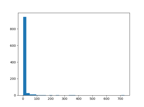
The answer is no. I wrote a script to search for a counterexample by generating random points on a sphere. Here’s one of the examples it came up with.

    x = [−0.9289  −0.0013   0.3704]
    y = [−0.8257   0.3963   0.4015]
    z = [−0.6977   0.7163  −0.0091]

Let d₁ = 1 − cossim(x, y), d₂ = 1 − cossim(y, z), and d₃ be 1 − cossim(x, z).

Then d₁ = 0.0849, d₂ = 0.1437, and d₃ = 0.3562 and so d₃ > d₁ + d₂.

Triangle inequality

The triangle inequality does hold if we work with θs rather than their cosines. The angle θ between two vectors is the distance between these two vectors interpreted as points on a sphere and the triangle inequality does hold on the sphere.

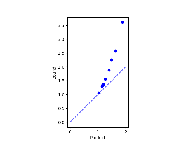
Approximate triangle inequality

If the cosine similarity between x and y is close to 1, and the cosine similarity between y and z is close to 1, then the cosine similarity between x and z is close to one, though the triangle inequality may not hold. I wrote about this before in the post Nearly parallel is nearly transitive.

I wrote in that post that the law of cosines for spherical trigonometry says

cos c = cos a cos b + sin a sin b cos γ

where γ is the angle between the arcs a and b. If cos a = 1 − ε₁, and cos b = 1 − ε₂, then

cos a cos b = (1 − ε₁)(1 − ε₂) = 1 − ε₁ − ε₂ + ε₁ ε₂

If ε₁ and ε₂ are small, then their product is an order of magnitude smaller. Also, the term

sin a sin b cos γ

is of the same order of magnitude. So if 1 − cossim(x, y) = ε₁ and 1 − cossim(y, z) = ε₂ then

1 − cossim(x, z) = ε₁ + ε₁ + O(ε₁ ε₂)

Is the triangle inequality desirable?

Cosine similarity does not satisfy the triangle inequality, but do we want a measure of similarity between words to satisfy the triangle inequality? You could argue that semantic similarity isn’t transitive. For example, lion is similar to king in that a lion is a symbol for a king. And lion is similar to house cat in that both are cats. But king and house cat are not similar. So the fact that cosine similarity does not satisfy the triangle inequality might be a feature rather than a bug.

Lehman’s inequality, circuits, and LaTeX

Posted on 6 July 2023 by John

Let A, B, C, and D be positive numbers. Then Lehman’s inequality says

$\frac{(A+B)(C+D)}{A+B+C+D} \geq \frac{AC}{A+C} + \frac{BD}{B+D}$

Proof by circuit

This inequality can be proved analytically, but Lehman’s proof is interesting because he uses electrical circuits [1].

Let A, B, C, and D be the resistances of resistors arranges as in the circuit on the left.

Resistors R₁ and R₂ in series have a combined resistance of

and the same resistors in parallel have a combined resistance of

$R = \frac{R_1 R_2}{R_1 + R_2}$

This means the circuit on the left has combined resistance

$\frac{(A+B)(C+D)}{A+B+C+D}$

The resistance of the circuit on the right is

$\frac{AC}{A+C} + \frac{BD}{B+D}$

Adding a short cannot increase resistance, so the resistance of the circuit on the right must be the same or lower than the resistance of the one on the left. Therefore

$\frac{(A+B)(C+D)}{A+B+C+D} \geq \frac{AC}{A+C} + \frac{BD}{B+D}$

Drawing circuits in LaTeX

I drew the circuits above using the circuitikz package in LaTeX. Here’s the code to draw the circuit on the left.

    \documentclass{article}
    
    \usepackage{tikz}
    \usepackage{circuitikz}
    
    \begin{document}
    
    \begin{figure}[h!]
      \begin{center}
        \begin{circuitikz}
          \draw (0,0)
          to[R=$B$] (0,2) 
          to[R=$A$] (0,4)
          to[short] (2,4) 
          to[R=$C$] (2,2)
          to[R=$D$] (2,0)
          to[short] (0,0);
          \draw (1,4)
          to[short] (1, 5);
          \draw (1, 0)
          to[short] (1, -1);
          %\draw (0, 2)
          %to[short] (2, 2);
        \end{circuitikz}
      \end{center}
    \end{figure}
    
    \end{document}

The code to draw the second circuit removes the %’s commenting out the code that draws the short between the two parallel arms of the circuit.

[1] Alfred Lehman proves a more general result using circuits in SIAM Review, Vol. 4, No. 2 (April 1962) pp. 150–151. Fazlollah Reza gives a purely mathematical proof on pages 151 and 152 of the same journal.

Strengthen Markov’s inequality with conditional probability

Posted on 23 March 2023 by John

Markov’s inequality is very general and hence very weak. Assume that X is a non-negative random variable, a > 0, and X has a finite expected value, Then Markov’s inequality says that

$\text{P}(X > a) \leq \frac{\text{E}(X)}{a}$

In [1] the author gives two refinements of Markov’s inequality which he calls Hansel and Gretel.

Hansel says

$\text{P}(X > a) \leq \frac{\text{E}(X)}{a + \text{E}(X - a \mid X > a)}$

and Gretel says

$\text{P}(X > a) \leq \frac{\text{E}(X) - \text{E}(X \mid X \leq a)}{a - \text{E}(X \mid X \leq a)}$

[1] Joel E. Cohen. Markov’s Inequality and Chebyshev’s Inequality for Tail Probabilities: A Sharper Image. The American Statistician, Vol. 69, No. 1 (Feb 2015), pp. 5-7

Inequalities for inequality: Gini coefficient lower bounds

Posted on 20 October 2022 by John

The Gini coefficient, a.k.a. Gini index, of a set of numbers is the average of all differences divided by twice the mean. Specifically, let

${\cal X} = \{x_1, x_2, x_3, \ldots, x_n\}$

Then the Gini coefficient of x is defined to be

$G({\cal X}) = \frac{1}{2\mu n^2} \sum_{i=1}^n \sum_{j=1}^n |x_i − x_j|$
where μ is the mean of the set. The Gini coefficient is often used in economics to measure inequalities in wealth.

Now suppose the data is divided into r disjoint groups:

${\cal X} = \bigcup_{i = 1}^r {\cal X}_i$

We would like to estimate the Gini coefficient of the entire group from Gini coefficients of each subgroup. This individual Gini coefficients alone are not enough data for the task, but if we also know the size and sum of each subgroup, we can compute lower bounds on G. The paper [1] gives five such lower bounds.

We will present the five lower bounds and see how well each does in a simulation.

Zagier’s lower bounds

Here are Zagier’s five lower bounds, listed in Theorem 1 of [1].

$\begin{align*} G({\cal X}) &\geq \sum_{i=1}^r \frac{n_i}{n} G({\cal X}_i) \\ G({\cal X}) &\geq \sum_{i=1}^r \frac{X_i}{X} G({\cal X}_i) \\ G({\cal X}) &\ge \left(\sum_{i=1}^r \sqrt{\frac{n_i}{n} \frac{X_i}{X} G({\cal X}_i)} \right)^2 \\ G({\cal X}) &\geq 1 - \left(\sum_{i=1}^r \sqrt{\frac{n_i}{n} \frac{X_i}{X} (1- G({\cal X}_i))} \right)^2 \\ G({\cal X}) &\geq G_0 = \sum_{i=1}^r \frac{n_i}{n} \frac{X_i}{X} G({\cal X}_i) \end{align*}$

Here n_i is the size of the ith subgroup and X_i is the sum of the elements in the ith subgroup. Also, n is the sum of the n_i and X is the sum of the X_i.

G₀ is the Gini coefficient we would get if we replaced each subgroup with its mean, eliminating all variance within subgroups.

Simulation

I drew 102 samples from a uniform random variable and computed the Gini coefficient with

    def gini(x):
        n = len(x)
        mu = sum(x)/n    
        s = sum(abs(a-b) for a in x for b in x)
        return s/(2*mu*n**2)

I split the sample evenly into three subgroups. I then sorted the list of samples and divided into three even groups again.

The Gini coefficient of the entire data set was 0.3207. The Gini coefficients of the three subgroups were 0.3013, 0.2798, and 0.36033. When I divided the sorted data into three groups, the Gini coefficients were 0.3060, 0.0937, and 0.0502. The variation in each group is the same, but the smallest group has a smaller mean and thus a larger Gini coefficient.

When I tested Zagier’s lower bounds on the three unsorted partitions, I got estimates of

[0.3138, 0.3105, 0.3102, 0.3149, 0.1639]

for the five estimators.

When I repeated this exercise with the sorted groups, I got

[0.1499, 0.0935, 0.0933, 0.1937, 0.3207]

The bounds for the first four estimates were much better for the unsorted partition, but the last estimate was better for the sorted partition.

Mahler’s inequality

Posted on 9 August 2022 by John

I ran across a reference to Mahler the other day, not the composer Gustav Mahler but the mathematician Kurt Mahler, and looked into his work a little. A number of things have been named after Kurt Mahler, including Mahler’s inequality.

Mahler’s inequality says the geometric mean of a sum bounds the sum of the geometric means. In detail, the geometric mean of a list of n non-negative real numbers is the nth root of their product. If x and y are two vectors of length n containing non-negative components, Mahler’s inequality says

G(x + y) ≥ G(x) + G(y)

where G is the geometric mean. The left side is strictly larger than the right unless x and y are proportional, or x and y both have a zero component in the same position.

I’m curious why this inequality is named after Mahler. The classic book Inequalities by Hardy, Littlewood, and Polya list the inequality but call it Hölder’s inequality. In a footnote they note that the inequality above appears in a paper by Minkowski in 1896 (seven years before Kurt Mahler was born). Presumably the authors file the inequality under Hölder’s name because it follows easily from Hölder’s inequality.

I imagine Mahler made good use of his eponymous inequality, i.e. that the inequality became associated with him because he applied it well rather than because he discovered it.

Reversed Cauchy-Schwarz inequality

Posted on 21 June 2021 by John

This post will state a couple forms of the Cauchy-Schwarz inequality and then present the lesser-known reverse of the Cauchy-Schwarz inequality due to Pólya and Szegö.

Cauchy-Schwarz inequality

The summation form of the Cauchy-Schwarz inequality says that

$\left( \sum_{n=1}^N x_n y_n \right)^2 \leq \left(\sum_{n=1}^N x_n^2\right) \left(\sum_{n=1}^N y_n^2\right)$

for sequences of real numbers x_n and y_n.

The integral form of the Cauchy-Schwarz inequality says that

$\left( \int_E f g\,d\mu \right)^2 \leq \left(\int_E f^2\,d\mu\right) \left(\int_E g^2 \,d\mu\right)$

for any two real-valued functions f and g over a measure space (E, μ) provided the integrals above are defined.

You can derive the sum form from the integral form by letting your measure space be the integers with counting measure. You can derive the integral form by applying the sum form to the integrals of simple functions and taking limits.

Flipping Cauchy-Schwarz

The Cauchy-Schwarz inequality is well known [1]. There are reversed versions of the Cauchy-Schwarz inequality that not as well known. The most basic such reversed inequality was proved by Pólya and Szegö in 1925 and many variations on the theme have been proved ever sense.

Pólya and Szegö’s inequality says

$\left(\int_E f^2\,d\mu\right) \left(\int_E g^2 \,d\mu\right) \leq C \left( \int_E f g\,d\mu \right)^2$

for some constant C provided f and g are bounded above and below. The constant C does not depend on the functions per se but on their upper and lower bounds. Specifically, assume

$\begin{align*} 0 < m_f \leq f \leq M_f < \infty \\ 0 < m_g \leq g \leq M_g < \infty \end{align*}$

Then

$C = \frac{1}{4} \frac{(m+M)^2}{mM}$

where

$\begin{align*} m &= m_f\, m_g \\ M &= M_f\, M_g \\ \end{align*}$

Sometimes you’ll see C written in the equivalent form

$C = \frac{1}{4} \left( \sqrt{\frac{M}{m}} + \sqrt{\frac{m}{M}} \right)^2$

This way of writing C makes it clear that the constant only depends on m and M via their ratio.

Note that if f and g are constant, then the inequality is exact. So the constant C is best possible without further assumptions.

The corresponding sum form follows immediately by using counting measure on the integers. Or in more elementary terms, by integrating step functions that have width 1.

Sum example

Let x = (2, 3, 5) and y = (9, 8, 7).

The sum of the squares in x is 38 and the sum of the squares in y is 194. The inner product of x and y is 18+24+35 = 77.

The product of the lower bounds on x and y is m = 14. The product of the upper bounds is M = 45. The constant C = 59²/(4×14×45) = 1.38.

The left side of the Pólya and Szegö inequality is 38×194 = 7372. The right side is 1.38×77²= 8182.02, and so the inequality holds.

Integral example

Let f(x) = 3 + cos(x) and let g(x) = 2 + sin(x). Let E be the interval [0, 2π].

The following Mathematica code shows that the left side of the Pólya and Szegö inequality is 171π² and the right side is 294 π².

The function f is bound below by 2 and above by 4. The function g is bound below by 1 and above by 3. So m = 2 and M = 12.

    In[1]:= f[x_] := 3 + Cos[x]
    In[2]:= g[x_] := 2 + Sin[x]
    In[3]:= Integrate[f[x]^2, {x, 0, 2 Pi}] Integrate[g[x]^2, {x, 0, 2 Pi}]
    Out[3]= 171 π²
    In[4]:= {m, M} = {2, 12};
    In[5]:= c = (m + M)^2/(4 m M);
    In[6]:= c Integrate[f[x] g[x], {x, 0, 2 Pi}]^2
    Out[6]= 294 π²

[1] The classic book on inequalities by Hardy, Littlewood, and Pólya mentions the Pólya-Szegö inequality on page 62, under “Miscellaneous theorems and examples.” Maybe Pólya was being inappropriately humble, but it’s odd that his inequality isn’t more prominent in his book.

Expected value of X and 1/X

Posted on 3 October 2020 by John

Yesterday I blogged about an exercise in the book The Cauchy-Schwarz Master Class. This post is about another exercise from that book, exercise 5.8, which is to prove Kantorovich’s inequality.

Assume

$0 < m \leq x_1 \leq x_2 \leq \cdots \leq x_n \leq M < \infty$

and

$p_1 + p_2 + \cdots + p_n = 1$

for non-negative numbers p_i.

Then

$\left(\sum_{i=1}^n p_i x_i \right) \left(\sum_{i=1}^n p_i \frac{1}{x_i} \right) \leq \frac{\mu^2}{\gamma^2}$

where

$\mu = \frac{m+M}{2}$

is the arithmetic mean of m and M and

$\gamma = \sqrt{mM}$

is the geometric mean of m and M.

In words, the weighted average of the x‘s times the weighted average of their reciprocals is bounded by the square of the ratio of the arithmetic and geometric means of the x‘s.

Probability interpretation

I did a quick search on Kantorovich’s inequality, and apparently it first came up in linear programming, Kantorovich’s area of focus. But when I see it, I immediately think expectations of random variables. Maybe Kantorovich was also thinking about random variables, in the context of linear programming.

The left side of Kantorovich’s inequality is the expected value of a discrete random variable X and the expected value of 1/X.

To put it another way, it’s a relationship between E[1/X] and 1/E[X],

$\text{E}\left(\frac{1}{X} \right ) \leq \frac{\mu^2}{\gamma^2} \frac{1}{\text{E}(X)}$

which I imagine is how it is used in practice.

I don’t recall seeing this inequality used, but it could have gone by in a blur and I didn’t pay attention. But now that I’ve thought about it, I’m more likely to notice if I see it again.

Python example

Here’s a little Python code to play with Kantorovich’s inequality, assuming the random values are uniformly distributed on [0, 1].

    from numpy import random

    x = random.random(6)
    m = min(x)
    M = max(x)
    am = 0.5*(m+M)
    gm = (m*M)**0.5
    prod = x.mean() * (1/x).mean()
    bound = (am/gm)**2
    print(prod, bound)

This returned 1.2021 for the product and 1.3717 for the bound.

If we put the code above inside a loop we can plot the product and its bound to get an idea how tight the bound is typically. (The bound is perfectly tight if all the x’s are equal.) Here’s what we get.

All the dots are above the dotted line, so we haven’t found an exception to our inequality.

(I didn’t think that Kantorovich had made a mistake. If he had, someone would have noticed by now. But it’s worth testing a theorem you know to be true, in order to test that your understanding of the theorem is correct.)

More inequalities

The baseball inequality

Posted on 2 October 2020 by John

baseball game

There’s a theorem that’s often used and assumed to be true but rarely stated explicitly. I’m going to call it “the baseball inequality” for reasons I’ll get to shortly.

Suppose you have two lists of k positive numbers each:

$n_1, n_2, n_3, \ldots, n_k$

and

$d_1, d_2, d_3, \ldots, d_k$

Then

$\min_{1 \leq i \leq k} \frac{n_i}{d_i} \leq \frac{n_1 + n_2 + n_3 + \cdots + n_k}{d_1 + d_2 + d_3 + \cdots + d_k} \leq \max_{1 \leq i \leq k} \frac{n_i}{d_i}$

This says, for example, that the batting average of a baseball team is somewhere between the best individual batting average and the worst individual batting average.

The only place I can recall seeing this inequality stated is in The Cauchy-Schwarz Master Class by Michael Steele. He states the inequality in exercise 5.1 and gives it the batting average interpretation. (Update: This is known as the “mediant inequality.” Thanks to Tom in the comments for letting me know. So the thing in the middle is called the “mediant” of the fractions.)

Note that this is not the same as saying the average of a list of numbers is between the smallest and largest numbers in the list, though that’s true. The batting average of a team as a whole is not the same as the average of the individual batting averages on that team. It might happen to be, but in general it is not.

I’ll give a quick proof of the baseball inequality. I’ll only prove the first of the two inequalities. That is, I’ll prove that the minimum fraction is no greater than the ratio of the sums of numerators and denominators. Proving that the latter is no greater than the maximum fraction is completely analogous.

Also, I’ll only prove the theorem for two numerators and two denominators. Once you have proved the inequality for two numerators and denominators, you can bootstrap that to prove the inequality for three numerators and three denominators, and continue this process for any number of numbers on top and bottom.

So we start by assuming

$\frac{a}{b} \leq \frac{c}{d}$

Then we have

$\begin{align*} \frac{a}{b} &= \frac{a\left(1 + \dfrac{d}{b} \right )}{b\left(1 + \dfrac{d}{b} \right )} \\ &= \frac{a + \dfrac{a}{b}d}{b + d} \\ &\leq \frac{a + \dfrac{c}{d}d}{b+d} \\ &= \frac{a + c}{b+d} \end{align*}$

Hadamard’s upper bound on determinant

Posted on 22 July 2020 by John

For an n by n real matrix A, Hadamard’s upper bound on determinant is

$|A|^2 \leq \prod_{i=1}^n \sum_{j=1}^n a_{ij}^2$

where a_ij is the element in row i and column j. See, for example, [1].

How tight is this upper bound? To find out, let’s write a little Python code to generate random matrices and compare their determinants to Hadamard’s bounds. We’ll take the square root of both sides of Hadamard’s inequality to get an upper bound on the absolute value of the determinant.

Hadamard’s inequality is homogeneous: multiplying the matrix A by λ multiplies both sides by λⁿ. We’ll look at the ratio of Hadamard’s bound to the exact determinant. This has the same effect as generating matrices to have a fixed determinant value, such as 1.

    
    from scipy.stats import norm
    from scipy.linalg import det
    import matplotlib.pyplot as plt
    import numpy as np
    
    # Hadamard's upper bound on determinant squared
    def hadamard(A):
        return np.prod(np.sum(A**2, axis=1))
                
    N = 1000
    ratios = np.empty(N)
    
    dim = 3
    for i in range(N):
        A = norm.rvs(size=(dim, dim))
        ratios[i] = hadamard(A)**0.5/abs(det(A))
    
    plt.hist(ratios, bins=int(N**0.5))
    plt.show()

In this simulation the ratio is very often around 25 or less, but occasionally much larger, 730 in this example.

histogram

It makes sense that the ratio could be large; in theory the ratio could be infinite because the determinant could be zero. The error is frequently much smaller than the histogram might imply since a lot of small values are binned together.

I modified the code above to print quantiles and ran it again.

    print(min(ratios), max(ratios))
    qs = [0.05, 0.25, 0.5, 0.75, 0.95]
    print( [np.quantile(ratios, q) for q in qs] )

This printed

    1.0022 1624.9836
    [1.1558, 1.6450, 2.6048, 5.7189, 32.49279]

So while the maximum ratio was 1624, the ratio was less than 2.6048 half the time, and less than 5.7189 three quarters of the time.

Hadamard’s upper bound can be very inaccurate; there’s no limit on the relative error, though you could bound the absolute error in terms of the norm of the matrix. However, very often the relative error is moderately small.

Convex function of diagonals and eigenvalues

Posted on 18 June 2020 by John

Sam Walters posted an elegant theorem on his Twitter account this morning. The theorem follows the pattern of an equality for linear functions generalizing to an inequality for convex functions. We’ll give a little background, state the theorem, and show an example application.

Let A be a real symmetric n×n matrix, or more generally a complex n×n Hermitian matrix, with entries a_ij. Note that the diagonal elements a_ii are real numbers even if some of the other entries are complex. (A Hermitian matrix equals its conjugate transpose, which means the elements on the diagonal equal their own conjugate.)

A general theorem says that A has n eigenvalues. Denote these eigenvalues λ₁, λ₂, …, λ_n.

It is well known that the sum of the diagonal elements of A equals the sum of its eigenvalues.

$\sum_{i=1}^n a_{ii} = \sum_{i=1}^n \lambda_i$

We could trivially generalize this to say that for any linear function φ: R → R,

$\sum_{i=1}^n \varphi(a_{ii}) = \sum_{i=1}^n \varphi({\lambda_i})$

because we could pull any shifting and scaling constants out of the sum.

The theorem Sam Walters posted says that the equality above extends to an inequality if φ is convex.

$\sum_{i=1}^n \varphi(a_{ii}) \leq \sum_{i=1}^n \varphi({\lambda_i})$

Here’s an application of this theorem. Assume the eigenvalues of A are all positive and let φ(x) = – log(x). Then φ is convex, and

$-\sum_{i=1}^n \log(a_{ii}) \leq -\sum_{i=1}^n \log({\lambda_i})$

and so

$\prod_{i=1}^n a_{ii} \geq \prod_{i=1}^n \lambda_i = \det(A)$

i.e. the product of the diagonals of A is an upper bound on the determinant of A.

This post illustrates two general principles:

Linear equalities often generalize to convex inequalities.
When you hear a new theorem about convex functions, see what it says about exp or −log.

Inequalities

Cosine similarity does not satisfy the triangle inequality

Counterexample

Triangle inequality

Approximate triangle inequality

Is the triangle inequality desirable?

Related posts

Lehman’s inequality, circuits, and LaTeX

Proof by circuit

Drawing circuits in LaTeX

Strengthen Markov’s inequality with conditional probability

Related posts

Inequalities for inequality: Gini coefficient lower bounds

Zagier’s lower bounds

Simulation

More posts on inequalities

Mahler’s inequality

More geometric mean posts

Reversed Cauchy-Schwarz inequality

Cauchy-Schwarz inequality

Flipping Cauchy-Schwarz

Sum example

Integral example

Related posts

Expected value of X and 1/X

Probability interpretation

Python example

More inequalities

The baseball inequality

More inequality posts

Hadamard’s upper bound on determinant

More posts on determinants

Convex function of diagonals and eigenvalues

More linear algebra posts