Charles Dodgson, better known by his pen name Lewis Carroll, discovered a method of calculating determinants now known variously as the method of contractants, Dodgson condensation, or simply condensation.

The method was devised for ease of computation by hand, but it has features that make it a practical method for computation by machine.

Overview

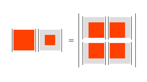
The basic idea is to repeatedly condense a matrix, replacing it by a matrix with one less row and one less column. Each element is replaced by the determinant of the 2×2 matrix formed by that element and its neighbors to the south, east, and southeast. The bottom row and rightmost column have no such neighbors and are removed. There is one additional part of the algorithm that will be easier to describe after introducing some notation.

Details

Let A be the matrix whose determinant we want to compute and let A^(k) be the matrix obtained after k steps of the condensation algorithm.

The matrix A⁽¹⁾ is computed as described in the overview:

Starting with A⁽²⁾ the terms are similar, except each 2×2 determinant is divided by an element from two steps back:

Dodgson’s original paper from 1867 is quite readable, surprisingly so given that math notation and terminology changes over time.

One criticism I have of the paper is that it is hard to understand which element should be in the denominator, whether the subscripts should be i and j or i+1 and j+1. His first example doesn’t clarify this because these elements happen to be equal in the example.

Example

Here’s an example using condensation to find the determinant of a 4×4 matrix.

We can verify this with Mathematica:

    Det[{{3, 1, 4, 1}, {5, 9, 2, 6}, 
         {0, 7, 1, 0}, {2, 0, 2, 3}}]

which also produces 228.

Division

The algorithm above involves a division and so we should avoid dividing by zero. Dodgson says to

Arrange the given block, if necessary, so that no ciphers [zeros] occur in its interior. This may be done either by transposing rows or columns, or by adding to certain rows the several terms of other rows multiplied by certain multipliers.

He expands on this remark and gives examples. I’m not sure whether this preparation is necessary only to avoid division by zero, but it does avoid the problem of dividing by a zero.

If the original matrix has all integer entries, then the division in Dodgson’s condensation algorithm is exact. The sequence of matrices produced by the algorithm will all have integer entries.

Efficiency

Students usually learn cofactor expansion as their first method of calculating determinants. This rule is easy to explain, but inefficient since the number of steps required is O(n!).

The more efficient way to compute determinants is by Gaussian elimination with partial pivoting. As with condensation, one must avoid dividing by zero, hence the partial pivoting.

Gaussian elimination takes O(n³) operations, and so does Dodgson’s condensation algorithm. Condensation is easy to teach and easy to carry out by hand, but unlike cofactor expansion it scales well.

If a matrix has all integer entries, Gaussian elimination can produce non-integer values in intermediate steps. Condensation does not. Also, condensation is inherently parallelizable: each of the 2 × 2 determinants can be calculated simultaneously.

Related posts

• Cofactors, determinants, and adjugates
• Why determinants with a column of 1s?
• Applied linear algebra

An elegant algebraic identity says

If x is the vector [a b] and y is the vector [c d] then this identity can be written

where the dot indicates the usual dot product. I posted this on Twitter the other day.

Gram matrix

Now suppose that x and y are vectors of any length n. The matrix on the right hand side above is called the Gram matrix of x and y, and its determinant is called the Gram determinant or Gramian.

Correlation

Let θ be the angle between x and y in ℝⁿ. Then

where ⟨x, y⟩ is the dot product of x and y.

If x and y are data vectors with mean 0, then cos θ is their correlation. Since correlation is unaffected by scaling, we can scale y so that it has the same norm as x, i.e. ||x|| = ||y||. Then the Gram matrix G can be written in terms of cos θ:

Generalization

The idea of the Gram matrix generalizes to more than two vectors. If we have m vectors, the Gram matrix is m × m whose (i, j) entry is the dot product of the ith and jth vectors. Note that the dimension n of the vectors does not have to equal the dimension m of the Gram matrix.

Let B be the matrix whose columns are the vectors x_i. If the number of vectors m does equal the dimension of the vectors n then B^T B equals the Gram matrix.

and so

If m does not equal n then B^T B cannot equal G because the two matrices have different dimensions, though the determinants of the two matrices are equal. That is, the square of the m-dimensional volume of the span of the x‘s inside ℝⁿ equals their Gram determinant.

The Gram determinant can be defined for more general inner products than the dot product in ℝⁿ. It could be, for example, the integral of the product of two functions.

Related posts

• Cofactors, determinants, and adjugates
• Circulant matrices commute
• Applied linear algebra

Here’s something I found surprising: the powers of a 2×2 matrix have a fairly simple closed form. Also, the derivation is only one page [1].

Let A be a 2×2 matrix with eigenvalues α and β. (3Blue1Brown made a nice jingle for finding the eigenvalues of a 2×2 matrix.)

If α = β then the nth power of A is given by

If α ≠ β then the nth power of A is given by

Example

Let’s do an example with

The eigenvalues are 26 and 3. I chose the matrix entries based on today’s date, not to have integer eigenvalues, and was surprised that they turned out so simple [2]. (More along those lines here.)

Here’s a little Python code to show that the formula above gives the same result as directly computing the cube of A.

    import numpy as np
    
    A = np.matrix([[6, 3], [20, 23]])
    m = (6 + 23)/2
    p = 6*23 - 3*20
    α = m + (m**2 - p)**0.5
    β = m - (m**2 - p)**0.5
    print(α, β)
    
    I = np.eye(2)
    direct = A*A*A
    
    formula = α**3*(A - β*I)/(α - β) + β**3*(A - α*I)/(β - α)
    print(direct)
    print(formula)

[1] Kenneth S. Williams. The nth Power of a 2×2 Matrix. Mathematics Magazine, Dec., 1992, Vol. 65, No. 5, p. 336.

[2] I wrote a script to find out how often this happens, and it’s more often than I would have guessed. There are 31 dates this year that would give integer eigenvalues if arranged as in the example.

Let A be an n × n matrix over a field F. The cofactor of an element A_ij is the matrix formed by removing the ith row and jth column, denoted A_{[i, j]}.

This terminology is less than ideal. The matrix just described is called the cofactor of A_ij, but it would more accurately be called the cofactor of (i, j) because it does not depend on the matrix entry A_ij per se but rather its position in the matrix A. For example, if someone asked you what the cofactor of 7 is, you’d have to say “That depends. Where is the 7 located?”. But we will stick to standard terminology.

(I wrote a post about a similar phenomenon in statistical notation, but I can’t find it this morning. You can’t answer questions like “What is p(0.5)?” in statistics by without first asking “If you were to write 0.5 using a variable, would you write it as x, y, or θ?”)

You can compute the determinant of a matrix by taking the alternating sum of elements of a row (or column) multiplied by the determinants of their cofactors.

This is essentially Cramer’s rule. It suggests a recursive procedure for computing determinants which is theoretically useful, but only computationally useful for very small matrices.

The adjugate of A, written adj(A), is the transpose of the matrix formed by replacing the (i, j) element of A with an alternating sign times its cofactor [1].

As you might guess, the Mathematica command to compute the adjugate is Adjugate.

Note that “adjugate” is not a typo for “adjoint.” The adjoint of A (now) means something different. What we now call the adjugate was sometimes in the past called the adjoint. What we now call the adjoint is the (conjugate) transpose.

Here’s an application of the adjugate. Let A be a 3 × 3 matrix. Then the characteristic polynomial of A is

where tr denotes the trace, the sum of the diagonal elements of a matrix.

Since the trace only depends on the diagonal, you only need to compute the diagonal of a adjugate to use the equation above for the characteristic polynomial. And the alternating terms defining the adjugate are all positive on the diagonal. So the trace of the adjugate is the sum of the determinants of the cofactors of the diagonal: det A₁₁ + det A₂₂ + det A₃₃.

A few days ago I wrote that circulant matrices all have the same eigenvectors. This post will show that it follows that circulant matrices commute with each other.

Recall that a circulant matrix is a square matrix in which the rows are cyclic permutations of each other. If we number the rows from 0, then the kth row takes the last k rows of the top row and moves them to the front.

Numerical example

We can generate two random circulant matrices and confirm that they commute by modifying the Python code from the earlier post.

    np.random.seed(42)
    N = 6
    row = np.random.random(N)
    A = np.array([np.roll(row, i) for i in range(N)])
    row = np.random.random(N)
    B = np.array([np.roll(row, i) for i in range(N)])
    AB = np.matmul(A, B)
    BA = np.matmul(B, A)
    print(np.absolute(AB - BA).max())

This computes two random 6 by 6 circulant matrices A and B and shows that the difference between AB and BA is on the order of the limit of floating point precision. Specifically, this prints 4.44 × 10⁻¹⁶.

Proof

Now for a proof. Let A and B be two matrices of size n that have the same set of independent eigenvectors e₁ through e_n. In the case of circulant matrices we can take e_k to be the kth column of the FFT matrix, but the proof here applies to any matrices with common eigenvectors.

Let α_k be the eigenvalue for e_k as an eigenvector of A and let β_k be the eigenvalue for e_k as an eigenvector of B. Then

and

and so multiplying by AB or BA has the same effect on e_k since the complex numbers α_k and β_k commute. Since the eigenvalues form a basis, and multiplication by AB and BA has the same effect on each basis vector, AB = BA.

In short, matrices that share eigenvectors commute because eigenvalues commute.

This post will look at rotating a matrix 90° and what that does to the determinant. This post was motivated by the previous post. There I quoted a paper that had a determinant with 1s in the right column. I debated rotating the matrix so that the 1s would be along the top because that seems more natural, but in the end I kept the original notation. If I had rotated the matrix, I’d need to adjust the value of the determinant.

Rotating a matrix is a an unusual operation. When someone speaks of turning a matrix over, they usually mean taking the transpose; taking the transpose is a reflection, not a rotation. And when you see the words “rotation” and “matrix” in close proximity, the topic is a matrix that represents a rotation. That’s not what this post is about: the matrix isn’t performing a rotation; a rotation is being performed on it.

Here’s an example:

Using subscripts makes the example above a little harder to read but much easier to formalize.

If we denote a matrix by A and its image after rotation as A‘, then the components a‘ of A‘ are related to the components a of A by

To form the rotation of A, we take the transpose of A, then reverse the order of the rows. In matrix notation,

where J is the matrix that has 1’s on the secondary diagonal, the diagonal running southwest to northeast, and 0’s everywhere else. The matrix J is the rotation of the identity matrix I.

The determinant of A‘ is the determinant of J times the determinant of A^T, and the determinant of A^T is the same as the determinant of A.

So the last thing we need to do to compute the determinant of A‘ is to compute the determinant of J.

We can turn I into J, and vice versa, by reversing the order of the rows. Let’s do this one pair of rows at a time. We swap the first and last rows. Then we swap the second row with the second to last row, then swap the third row from the top with the third row from the bottom, etc.

Suppose I is an n × n matrix, and first assume n is even. Then we need to do n/2 swaps, swapping each of the top n/2 rows with one of the bottom n/2 rows. Each swap reverses the sign of the determinant, and so the determinant of J is (−1)^n/2. Now if n is odd, the middle row doesn’t move. So we swap the top (n − 1)/2 rows with the bottom (n − 1)/2 rows. So in that case the determinant of J is (−1)^(n−1)/2. We can combine the even and the odd case using floor notation: