Famous constants and the Gumbel distribution

The Gumbel distribution, named after Emil Julius Gumbel (1891–1966), is important in statistics, particularly in studying the maximum of random variables. It comes up in machine learning in the so-called Gumbel-max trick. It also comes up in other applications such as in number theory.

For this post, I wanted to point out how a couple famous constants are related to the Gumbel distribution.

Gumbel distribution

The standard Gumbel distribution is most easily described by its cumulative distribution function

F(x) = exp( −exp(−x) ).

You can introduce a location parameter μ and scale parameter β the usual way, replacing x with (x − μ)/β and dividing by β.

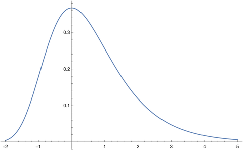
Here’s a plot of the density.

Euler-Mascheroni constant γ

The Euler-Mascheroni constant γ comes up frequently in applications. Here are five posts where γ has come up.

The constant γ comes up in the context of the Gumbel distribution two ways. First, the mean of the standard Gumbel distribution is γ. Second, the entropy of a standard Gumbel distribution is γ + 1.

Apéry’s constant ζ(3)

The values of the Riemann zeta function ζ(z) at positive even integers have closed-form expressions given here, but the values at odd integers do not. The value of ζ(3) is known as Apéry’s constant because Roger Apéry proved in 1978 that ζ(3) is irrational.

Like the Euler-Mascheroni constant, Apéry’s constant has come up here multiple times. Some examples:

The connection of the Gumbel distribution to Apéry’s constant is that the skewness of the distribution is

12√6 ζ(3)/π³.

Prime numbers and Taylor’s law

The previous post commented that although the digits in the decimal representation of π are not random, it is sometimes useful to think of them as random. Similarly, it is often useful to think of prime numbers as being randomly distributed.

If prime numbers were samples from a random variable, it would be natural to look into the mean and variance of that random variable. We can’t just compute the mean of all primes, but we can compute the mean and variance of all primes less than an upper bound x.

Let M(x) be the mean of all primes less than x and let V(x) be the corresponding variance. Then we have the following asymptotic results:

M(x) ~ x / 2

and

V(x) ~ x²/12.

We can investigate how well these limiting results fit for finite x with the following Python code.

    from sympy import sieve
    
    def stats(x):
        s = 0
        ss = 0
        count = 0
        for p in sieve.primerange(x):
            s += p
            ss += p**2
            count += 1
        mean = s / count
        variance = ss/count - mean**2
        return (mean, variance)

So, for example, when x = 1,000 we get a mean of 453.14, a little less than the predicted value of 500. We get a variance of 88389.44, a bit more than the predicted value of 83333.33.

When x = 1,000,000 we get closer to values predicted by the limiting formula. We get a mean of 478,361, still less than the prediction of 500,000, but closer. And we get a variance of 85,742,831,604, still larger than the prediction 83,333,333,333, but again closer. (Closer here means the ratios are getting closer to 1; the absolute difference is actually getting larger.)

Taylor’s law

Taylor’s law is named after ecologist Lionel Taylor (1924–2007) who proposed the law in 1961. Taylor observed that variance and mean are often approximately related by a power law independent of sample size, that is

V(x) ≈ a M(x)b

independent of x.

Taylor’s law is an empirical observation in ecology, but it is a theorem when applied to the distribution of primes. According to the asymptotic results above, we have a = 1/3 and b = 2 in the limit as x goes to infinity. Let’s use the code above to look at the ratio

V(x) / a M(x)b

for increasing values of x.

If we let x = 10k for k = 1, 2, 3, …, 8 we get ratios

0.612, 1.392, 1.291, 1.207, 1.156, 1.124, 1.102, 1.087

which are slowly converging to 1.

Related posts

Reference: Joel E. Cohen. Statistics of Primes (and Probably Twin Primes) Satisfy Taylor’s Law from Ecology. The American Statistician, Vol. 70, No. 4 (November 2016), pp. 399–404

The coupon collector problem and π

How far do you have to go down the decimal digits of π until you’ve seen all the digits 0 through 9?

We can print out the first few digits of π and see that there’s no 0 until the 32nd decimal place.

3.14159265358979323846264338327950

It’s easy to verify that the remaining digits occur before the 0, so the answer is 32.

Now suppose we want to look at pairs of digits. How far out do we have to go until we’ve seen all pairs of digits (or base 100 digits if you want to think of it that way)? And what about triples of digits?

We know we’ll need at least 100 pairs, and at least 1000 triples, so this has gotten bigger than we want to do by hand. So here’s a little Python script that will do the work for us.

    from mpmath import mp
    
    mp.dps = 30_000
    s = str(mp.pi)[2:] 
    
    for k in [1, 2, 3]:
        tuples = [s[i:i+k] for i in range(0, len(s), k)]
        d = dict()
        i = 0
        while len(d) < 10**k:
            d[tuples[i]] = 1
            i += 1
        print(i)

The output:

    32
    396
    6076

This confirms that we at the 32nd decimal place we will have seen all 10 possible digits. It says we need 396 pairs of digits before we see all 100 possible digit pairs, and we’ll need 6076 triples before we’ve seen all possible triples.

We could have used the asymptotic solution to the “coupon collector problem” to approximately predict the results above.

Suppose you have an urn with n uniquely labeled balls. You randomly select one ball at a time, return the ball to the run, and select randomly again. The coupon collector problem ask how many draws you’ll have to make before you’ve selected each ball at least once.

The expected value for the number of draws is

n Hn

where Hn is the nth harmonic number. For large n this is approximately equal to

n(log n + γ)

where γ is the Euler-Mascheroni constant. (More on the gamma constant here.)

Now assume the digits of π are random. Of course they’re not random, but random is as random does. We can get useful estimates by making the modeling assumption that the digits behave like a random sequence.

The solution to the coupon collector problem says we’d expect, on average, to sample 28 digits before we see each digit, 518 pairs before we see each pair, and 7485 triples before we see each triple. “On average” doesn’t mean much since there’s only one π, but you could interpret this as saying what you’d expect if you repeatedly chose real numbers at random and looked at their digits, assuming the normal number conjecture.

The variance on the number of draws needed is asymptotically π² n²/6, so the number of draws with usually be an interval of the expected value ± 2n.

If you want the details of the coupon collector problem, not just the expected value but the probabilities for different number of draws, see Sampling with replacement until you’ve seen everything.


Numbering minor league baseball teams

El Paso Chihuahuas team logo
Last week I wrote about how to number MLB teams so that the number n told you where they are in the league hierarchy:

  • n % 2 tells you the league, American or National
  • n % 3 tells you the division: East, Central, or West
  • n % 5 is unique within a league/division combination.

Here n % m denotes n mod m, the remainder when n is divided by m.

This post will do something similar for minor league teams.

There are four minor league teams associated with each major league team. If we wanted to number them analogously, we’d need to do something a little different because we cannot specify n % 2 and n % 4 independently. We’d need an approach that is a hybrid of what we did for the NFL and MLB.

We could specify the league and the rank within the minor leagues by three bits: one bit for National or American league, and two bits for the rank:

  • 00 for A
  • 01 for High A
  • 10 for AA
  • 11 for AAA

It will be convenient later on if we make the ranks the most significant bits and the league the least significant bit.

So to place a minor league team on a list, we could write down the numbers 1 through 120, and for each n, calculate r = n % 8, d = n % 3, and k = n % 5.

The latest episode of 99% Invisible is called RoboUmp, a show about automating umpire calls. As part of the story, the show discusses the whimsical names of minor league teams and how the names allude to their location. For example, the El Paso Chihuahuas are located across the border from the Mexican state of Chihuahua and their mascot is a chihuahua dog. (The dog was named after the state.)

The El Paso Chihuahuas are the AAA team associated with the San Diego Padres, a team in the National League West, team #3 in the order listed in the MLB post. The number n for the Chihuahuas must equal 7 mod 8, 111two, the first bit for National League and the last two bits for AAA. We also require n to be 2 mod 3 because it’s in the West, and n = 3 mod 5 because the Padres are #3 in the list of National League West teams in our numbering. It works out that n = 23.

How do minor league and major league numbers relate? They have to be congruent mod 30. They have to have the same parity since they represent the same league, and must be congruent mod 3 because they have in the same division. And they must be congruent mod 5 to be in the same place in the list of associated major league teams.

So to calculate a minor league team’s number, start with the corresponding major league number, and add multiples of 30 until you get the right value mod 8.

For example, the Houston Astros are number 20 in the list from the earlier post. The Triple-A team associated with the Astros is the Sugar Land Space Cowboys. The number n for the Space Cowboys must be 6 mod 8 because 6 = 110two, and they’re a Triple-A team (11) in the American League (0). So n = 110.

The Astros’ Double-A team, the Corpus Christi Hooks, needs to have a number equal to 100two = 4 mod 8, so n = 20. The High-A team, the Asheville Tourists, are 50 and the Single-A team, the Fayetteville Woodpeckers, is 80.

You can determine what major league team is associated with a minor league team by taking the remainder by 30. For example, the Rocket City Trash Pandas has number 77, so they’re associated with the major league team with number 17, which is the Los Angeles Angels. The remainder when 77 is divided by 8 is 5 = 101two, which tells you they’re a Double-A team since the high order bits are 1 and 0.

John Conway’s mental factoring method and friends

There are tricks for determining whether a number is divisible by various primes, but many of these tricks have to be applied one at a time. You can make a procedure for testing divisibility by any prime p that is easier than having to carry out long division, but these rules are of little use if every one of them is different.

Say I make a rule for testing whether a number is divisible by 59. That’s great, if you routinely need to test divisibility by 59. Maybe you work for a company that, for some bizarre reason, ships widgets in boxes of 59 and you frequently have to test whether numbers are multiples of 59.

When you want to factor numbers, you’d like to test divisibility by a set of primes at once, using fewer separate algorithms, and taking advantage of work you’ve already done.

John Conway came up with his 150 Method to test for divisibility by a sequence of small primes. This article explains how Conway’s 150 method and a couple variations work. The core idea behind Conway’s 150 Method, his 2000 Method, and analogous methods developed by others is this:

  1. Find a range of integers, near a round number, that contains a lot of distinct prime factors.
  2. Reduce your number modulo the round number, then test for divisibility sequentially, reusing work.

Conway’s 150 Method starts by taking the quotient and remainder by 150. And you’ll never guess what his 2000 Method does. :)

This post will focus on the pattern behind Conway’s method, and similar methods. For examples and practical tips on carrying out the methods, see the paper linked above and a paper I’ll link to below.

The 150 Method

Conway exploited the fact that the numbers 152 through 156 are divisible by a lot of primes: 2, 3, 5, 7, 11, 13, 17, 19, and 31.

He starts his method with 150 rather than 152 because 150 is a round number and easier to work with. We start by taking the quotient and remainder by 150.

Say n = 150q + r. Then n − 152q = r − 2q. If n has three or four digits, q only has one or two digits, and so subtracting q is relatively easy.

Since 19 divides 152, we can test whether n is divisible by 19 by testing whether r − 2q is divisible by 19.

The next step is where sequential testing saves effort. Next we want to subtract off a multiple of 153 to test for divisibility by 17, because 17 divides 153. But we don’t have to start over. We can reuse our work from the previous step.

We want n − 153q = (n − 152q) − q, and we’ve already calculated n − 152q in the previous step, so we only need to subtract q.

The next step is to find n − 154q, and that equals (n − 153q) − q, so again we subtract q from the result of the previous step. We repeat this process, subtracting q each time, and testing for divisibility by a new set of primes each time.

The 2000 method

Conway’s more extensive method exploited the fact that the numbers 1998 through 2021 are divisible by all primes up to 67. So he would start by taking the quotient and remainder by 2000, which is really easy to do.

Say n = 2000q + r. Then we would add (or subtract) q each time.

You could start with r, then test r for divisibility by the factors of 2000, then test rq for divisibility by the factors of 2001, then test r − 2q for divisibility by the factors of 2002, and so on up to testing r − 21q for divisibility by the factors of 2021. Then you’d need to go back and test r + q for divisibility by the factors of 1999 and test r + 2q for divisibility by the factors of 1998.

In principle that’s how Conways 2000 Method works. In practice, he did something more clever.

Most of the prime factors of the numbers 1998 through 2021 are prime factors of 1998 through 2002, so it makes sense to test this smaller range first hoping for early wins. Also, there’s no need to test divisibility by the factors of 1999 because 1999 is prime.

Conway tested rkq for k = −2 through 21, but not sequentially. He would try out the values of k in an order most likely to terminate the factoring process early.

The 10,000 method

This paper gives a much more extensive approach to mental factoring than Conway’s 150 method. The authors, Hilarie Orman and Richard Schroeppel, outline a strategy for factoring any six-digit number. Conway’s rule is more modest, intended for three and four digit numbers.

Orman and Schroeppel suggest a sequence of factoring methods, including more advanced techniques to use after you’ve tried testing for divisibility by small primes. One of the techniques in the paper might be called the 10,000 Method by analogy to Conway’s method, though the authors don’t call it that. They call it “check the m‘s” for reasons that make more sense if you read the paper.

The 10,000 Method is much like the 2000 Method. The numbers 10,001 through 10,019 have a lot of prime factors, and the method tests for divisibility by these factors sequentially, taking advantage of previous work at each step, just as Conway’s methods do. The authors do not backtrack the way Conway did; they test numbers in order. However, they do skip over some numbers, like Conway skipped over 1999.

More Conway-related posts
Major League Baseball and number theory

The previous post took a mathematical look at the National Football League. This post will do the same for Major League Baseball.

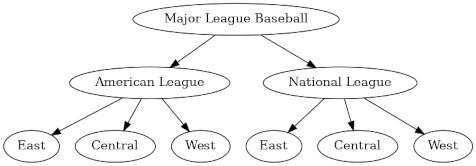
Like the NFL, MLB teams are organized into a nice tree structure, though the MLB tree is a little more complicated. There are 32 NFL teams organized into a complete binary tree, with a couple levels collapsed. There are 30 MLB teams, so the tree structure has to be a bit different.

MLB has leagues rather than conferences, but the top-level division is into American and Nation as with the NFL. So the top division is into the American League and the National League.

And as with football, the next level of the hierarchy is divisions. But baseball has three divisions—East, Central, and West—in contrast to four in football.

Each division has five baseball teams, while each football division has four teams.

Here’s the basic tree structure.

Under each division are five teams. Here’s a PDF with the full graph including teams.

Geography

How do the division names correspond to actual geography?

Within each league, the Central teams are to the west of the East teams and to the east of the West teams, with one exception: in the National League, the Pittsburgh Pirates are a Central division team, but they are east of the Atlanta Braves and Miami Marlins in the East division. But essentially the East, Central, and West divisions do correspond to geographic east, center, and west, within a league.

Numbering

We can’t number baseball teams as elegantly as the previous post numbered football teams. We’d need a mixed-base number. The leading digit would be binary, the next digit base 3, and the final digit base 5.

We could number the teams so that you could tell the league and division of the team by looking at the remainders when the number is divided by 2 and 3, and each team is unique mod 5. By the Chinese Remainder Theorem, we can solve the system of congruence equations mod 30 that specify the value of a number mod 2, mod 3, and mod 5.

If we number the teams as follows, then even numbered teams are in the American League and odd numbered teams are in the National League. When the numbers are divided by 3, those with remainder 0 are in an Eastern division, those with remainder 1 are in a Central division, and those with remainder 2 are in a Western division. Teams within the same league and division have unique remainders by 5.

  1. Cincinnati Reds
  2. Oakland Athletics
  3. Philadelphia Phillies
  4. Minnesota Twins
  5. Arizona Diamondbacks
  6. Boston Red Sox
  7. Milwaukee Brewers
  8. Seattle Mariners
  9. Washington Nationals
  10. Chicago Whitesocks
  11. Colorado Rockies
  12. New York Yankees
  13. Pittsburgh Pirates
  14. Texas Rangers
  15. Atlanta Braves
  16. Cleveland Guardians
  17. Los Angeles Dodgers
  18. Tampa Bay Rays
  19. St. Louis Cardinals
  20. Houston Astros
  21. Miami Marlins
  22. Detroit Tigers
  23. San Diego Padres
  24. Toronto Blue Jays
  25. Chicago Cubs
  26. Los Angeles Angels
  27. New York Mets
  28. Kansas City Royals
  29. San Francisco Giants
  30. Baltimore Orioles

Related posts

Divisibility by base + 1

To test whether a number is divisible by 11, add every other digit together and subtract the rest of the digits. The result is divisible by 11 if and only if the original number is divisible by 11.

For example, start with n = 31425. Add 3, 4, and 5, and subtract 1 and 2. Since 3 + 4 + 5 − 1 − 2 = 9, and 9 is not divisible by 11, neither is 31425.

For another example, take 349041. We have 3 + 9 + 4 = 16, and 4 + 0 + 1 = 5, and 16 − 5 = 11. Since 11 is obviously divisible by 11, so is 349041.

The same trick that works for testing base 10 numbers for divisibility by 11 works for testing base 16 numbers for divisibility by 17. More generally, it works for testing base b numbers for divisibility by b+1.

Let m = b + 1. Then

 b \equiv −1 \pmod m

which implies

\sum_{n=0}^N a_nb^n \equiv \sum_{n=0}^N a_n(-1)^n \pmod m

Here an is the nth digit of a number in base b, numbering the digits from the least significant, counting from 0.

Sometimes a rule for testing divisibility by m will also tell you the remainder when a number is divided by m, but sometimes not. The method presented here will give you the remainder by b + 1, but only if you start adding up digits from the right end. Note in the proof that the digits in even positions (counting from 0) have a positive coefficient and the digits in odd positions have a negative coefficient.

For example, let’s look at 1EDA86hex in hexadecimal (base 16). If we add 6, A, and E, and subtract 8, D, and 1, we get 8, which is the remainder when 1EDA86hex is divided by 11hex (i.e. 17ten). But if we add 1, D, and 8 and subtract E, A, and 8, we get 9.

You can start from either end of a number if you only want to test divisibility, not to compute a remainder. But if you do want the remainder, you might get the wrong result if you start at the wrong end.

Application: Divisibility by 7, 11, and 13

We can apply the technique above to test for divisibility by 1001 in base 1000. And why would we want to do that? Because 1001 = 7 × 11 × 13. Reducing a large number mod 1001 takes the problem of testing for divisibility mod 7, 11, or 13 down to the problem of testing 3-digit numbers.

Base 1000 is just base 10, thinking of triples of ordinary digits as a single base 1000 digit. If we write a number with thousands separators (i.e. commas in some countries, periods in others) then each segment is a base 1000 “digit.”

Example 1

For example, let’s test whether n = 598,203,918 is divisible by 7, 11, or 13.

The alternating (base 1000) digit sum is

598 − 203 + 918 = 1313 = 13 × 101.

The result is clearly divisible by 13, so n is divisible by 13. But since 101 is not divisible by 7 or 11, neither is n.

Example 2

For another example, let n = 314,159,265,358 and find the remainders when n is divided by 7, 11, and 13. We start by reducing n mod 1001.

314159265358 =  −314 + 159 − 265 + 358 = −62 = 939 mod 1001.

Now 939 = 1 = mod 7, so n = 1 mod 7.

Also, 9 + 9 − 3 = 15 = 4 mod 11, and so n = 4 mod 11.

Finally, 939 = 3 mod 13, so n = 3 mod 13.


Rotating multiples of 37

If a three-digit number is divisible by 37, it remains divisible by 37 if you rotate its digits. For example, 148 is divisible by 37, and so are 814 and 481. This rotation property could make it easier to recognize multiples of 37 or easier to carry out trial division.

Before proving the theorem, I’ll state a couple things the theorem does not say. First of all, it does not say that you can reverse the digits. For example, although 148 is divisible by 37, 841 is not. Second, it does not say that rotating digits preserves the remainder by 37 except when that remainder is 0. For example, 123 = 12 mod 37, but 312 = 16 mod 37.

Now for the proof. Let a, b, and c be integers. Let

n = 100a + 10b + c.

and assume that n is a multiple of 37. We want to show that

m = 100c + 10a + b

is also a multiple of 37. If we can prove this, then we can apply the result to m to obtain one more rotation.

Note that 999 = 27 × 37, so n + 999c is also a multiple of 37. Now

k = n + 999c = 1000c + 100a + 10b

is clearly divisible by 10, and 10 is relatively prime to 37, so k/10 must also be divisible by 37, and

k/10 = 100c + 10a + b

which is just the rotation we were looking for.

Note that to prove the theorem at the top of the post it is enough to assume a, b, and c are digits, but the proof is valid for any integer values.

Pythagorean triangles with side 2023

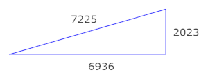
Can a Pythagorean triangle have one size of length 2023? Yes, one possibility is a triangle with sides (2023, 6936, 7225).

right triangle with sides 2023, 6936, and 7225

Where did that come from? And can we be more systematic, listing all Pythagorean triangles with a side of length 2023?

Euclid’s formula generates Pythagorean triples by sticking integers m and n into the formula

(m² – n², 2mn, m² + n²).

If one of these three numbers equals 2023, it’s going to have to be the first one. Why? The second number is even, and 2023 is odd, so that one is ruled out.

It’s less obvious but true that the hypotenuse m² + n² cannot be 2023. We could verify this by brute force, trying integer values of m between 1 and √2023, subtracting m² from 2023, and seeing whether the result is a square. But there is a more elegant approach.

There is a theorem that says an integer N is the sum of two squares exactly when every prime that divides N is either congruent to 1 mod 4 or appears an even number of times in the factorization of N. The prime factorization of N is 7 × 17 × 17. The factor 7 appears to an odd power and 7 = 3 mod 4.

Is 2023 a difference of squares? Yes, every odd number is a difference of squares.

To write an number N as a difference of squares, we have to solve

m² – n² = (m + n)(m – n) = N.

If N is odd, we can always set mn = 1. In the case N = 2023, this means m = 1012 and n = 1011.

The solution above corresponds to factoring 2023 as 2023 × 1. We could also factor 2023 as 289 × 7 or 119 × 17. (The first factor has to be larger than the second for mn to be positive.) To find more possible value of m and n we solve the equations

m + n = 289
mn = 7

and

m + n = 119
mn = 17.

These have solution (148, 141) and (68, 51).

To summarize, we can find three Pythagorean triples with one component equal to 2023 using Euclid’s formula. These are

(2023, 2046264, 2046265)
(2023, 41736, 41785)
(2023, 6936, 7225)

corresponding to (m, n) = (1013, 1012), (148, 141), and (68, 51) respectively. The first two are primitive Pythagorean triples because the three numbers are relative prime in both cases. The last triple is not primitive because each number is divisible by 289.

Euclid’s formula generates all primitive Pythagorean triples, but it doesn’t generate all possible Pythagorean triples. To find all Pythagorean triples we have to consider solutions of the form

(km² – kn², 2kmn, km² + kn²)

for some integer k. If 2023 is k times a difference of squares, k must be a factor of 2023, and so k = 1, 7, 17, 119, 289, or 2023. We’ve already considered the case k = 1.

For k = 7, we express 289 as a difference of squares. The only solutions with positive integers is (m, n) = (145, 144). This yields the Pythagorean triple

(2023, 292320, 292327).

For k = 17, we express 119 as a difference of squares. The solutions are (m, n) = (60, 59) and (12, 5). These yield

(2023, 120360, 120377)

and

(2023, 2040, 2873).

For k = 119, we express 17 as a difference of squares. This can only be done one way, (m, n) = (9, 8). This yields

(2023, 17136, 17255).

For k = 289, we express 7 as a difference of squares. The unique solution (4, 3) yields the triple

(2023, 6936, 7225)

that we had found previously.

For k = 2023, we have to write 1 as a difference of squares. This has no solution if we require both squares to be positive.

So we’re done. We’ve found all Pythagorean triples containing 2023.

Related posts

Factoring b^n + 1

The previous post illustrated a technique for finding factors of number of the form bn – 1. This post will look at an analogous, though slightly less general, technique for numbers of the form bn + 1.

There is a theorem that says that if m divides n then bm + 1 divides bn + 1 if n is odd. To see that the exponent must be odd, let b = 10, n = 4, and m = 2: 10,0001 is not divisible by 101.

Last time we looked at 22023 – 1, so this time let’s look at J = 22023 + 1.

Since 2023 = 7×17×17, we know J is divisible by 2n + 1 for n = 7, 17, 7×17, and 17×17. Factoring each of these factors tells us that J is divisible by

  • 3
  • 43691
  • 72251
  • 79187
  • 1077971
  • 823679683
  • 18360250452977
  • 197766803208315851
  • 143162553165560959297
  • 338858733065598401355195539629373089

(If it seems this post is moving too fast, you might want to go back and read the previous post and then come back.)

Let P be the product of the factors above, and let F = J/P.  Now F is a 493-digit number, so we don’t expect to be able to get much further unless we’re lucky. We can find three factors of F

  • 43
  • 4382432993
  • 1809032819104754041

but then we get stuck. We know there are more factors, but it seems doubtful that I’m going to find any more anytime soon.

***

As in the previous post, we’ll conclude with Python code to verify the claims above.

from sympy import isprime

def verify_factors(N, factors, full=True):
    prod = 1
    for f in factors:
        assert(isprime(f))
        prod *= f
    if full:
        assert(N == prod)
    else:
        assert(N % prod == 0)
        assert(not isprime(N // prod))
    return N // prod

factors = [
    3,
    43691,
    72251,
    79187,
    1077971,
    823679683,
    18360250452977,
    197766803208315851,
    143162553165560959297,
    338858733065598401355195539629373089
]

J = 2**2023 + 1
F = verify_factors(J, factors, False)

factors = [43, 4382432993, 1809032819104754041]
verify_factors(F, factors, False)

print(len(str(F)))