AI models hallucinate, and always will [1]. In some sense this is nothing new: everything has an error rate. But what is new is the nature of AI errors. The output of an AI is plausible by construction [2], and so errors can look reasonable even when they’re wrong. For example, if you ask for the capital city of Illinois, an AI might err by saying Chicago, but it wouldn’t say Seattle.
You need to decide two things when evaluating whether to use an AI for a task: the cost of errors and the cost of validation.
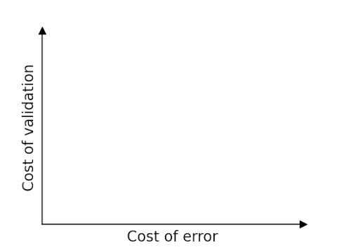
Image generation is an ideal task for AIs because the consequences of an error are usually low. And validation is almost effortless: if an image looks OK, it’s OK. So imagine generation is in the bottom left corner of the image above.
Text-to-speech is a little more interesting to evaluate. The consequences of an error depend on user expectations. Someone may be mildly annoyed when a computer makes an error reading an email out loud, but the same person may angry if he thought he was talking to a human and discovers he’s been talking to a machine.
Validating text-to-speech requires a human to listen to the audio. This doesn’t require much effort, though the cost might be too much in some contexts. (I’m in the middle of an AI-narrated book and wondering why the producer didn’t go to the effort of fixing the pronunciation errors. The print version of the book has high production quality, but not as much effort went into the audio.) So I’d say text-to-speech is somewhere in the bottom half of the graph, but the horizontal location depends on expectations.
Code generation could be anywhere on the graph, depending on who is generating the code and what the code is being used for. If an experienced programmer is asking AI to generate code that in principle he could have written, then it should be fairly easy to find and fix errors. But it’s not a good idea for a non-programmer to generate code for a safety-critical system.
Mitigating risks and costs
The place you don’t want to be is up and to the right: errors are consequential and validation is expensive. If that’s where your problem lies, then you want to either mitigate the consequences of errors or reduce the cost of validation.
This is something my consultancy helps clients with. We find ways to identify errors and to mitigate the impact of inevitable errors that slip through.
If you’d like help moving down and to the left, lowering the cost of errors and the cost of validation, let’s set up a meeting to discuss how we can help.
[1] LLMs have billions of parameters, pushing a trillion. But as large as the parameter space is, the space of potential prompts is far larger, and so the parameters do not contain enough information to respond completely accurately to every possible prompt.
[2] LLMs predict the word that is likely to come next given the words produced so far. In that sense, the output is always reasonable. If an output does not appear reasonable to a human, it is because the human has more context.