Extending harmonic numbers

For a positive integer n, the nth harmonic number is defined to be the sum of the reciprocals of the first n positive integers:

H_n = 1 + \frac{1}{2} + \frac{1}{3} + \cdots + \frac{1}{n}

How might we extend this definition so that n does not have to be a positive integer?

First approach

One way to extend harmonic numbers is as follows. Start with the equation

(t - 1)(t^{n-1} + t^{n-2} + t^{n-3} + \cdots + 1) = t^n - 1

Then

\frac{t^n - 1}{t-1} = t^{n-1} + t^{n-2} + t^{n-3} + \cdots + 1

Integrate both sides from 0 to 1.

\int_0^1\frac{t^n - 1}{t-1} \,dt = \frac{1}{n} + \frac{1}{n-1} + \frac{1}{n-2} + \cdots + 1 = H_n

So when x is an integer,

H_x = \int_0^1\frac{t^x - 1}{t-1} \,dt

is a theorem. When x is not an integer, we take this as a definition.

Second approach

Another approach is to start with the identity

\Gamma(x+1) = x\, \Gamma(x)

then take the logarithm and derivative of both sides. This gives

\psi(x+1) = \frac{1}{x} + \psi(x)

where the digamma function ψ is defined to be the derivative of the log of the gamma function.

If x is an integer and we apply the identity above repeatedly we get

\psi(n+1) = H_n + \psi(1) = H_n - \gamma

where γ is Euler’s constant. Then we can define

H_x = \psi(x + 1) + \gamma

for general values of x.

Are they equal?

We’ve shown two ways of extending the harmonic numbers. Are these two different extensions or are they equal? They are in fact equal, which follows from equation 12.16 in Whittaker and Watson, citing a theorem of Legendre.

Taking either approach as our definition we could, for example, compute the πth harmonic number (1.87274) or even the ith harmonic number (0.671866 + 1.07667i).

An addition rule

The digamma function satisfies an addition rule

\psi(2z) = \frac{1}{2} \left( \psi(z) + \psi\left(z + \frac{1}{2}\right)\right) + \log 2


which can be proved by taking the logarithm and derivative of Gauss’s multiplication rule for the gamma function.

Let z = x + 1/2 and add γ to both sizes. This shows that harmonic numbers satisfy the addition rule

H_{2x} = \frac{1}{2}\left( H_{x-1/2} + H_x \right) + \log 2

Related posts

When does a function have an addition theorem?

Motivating examples

The addition theorem for cosine says that

\cos(x + y) = \cos x \cos y - \sin x \sin y

and the addition theorem for hyperbolic cosine is analogous, though with a sign change.

\cosh(x + y) = \cosh x \cosh y + \sinh x \sinh y

An addition theorem is a theorem that relates a function’s value at x + y to its values at x and at y. The squaring function satisfies a very simple addition theorem

(x + y)^2 = x^2 + 2xy + y^2

and the Jacobi function sn satisfies a more complicated addition theorem.

\text{sn}(x + y) = \frac{ \text{cn}(x)\, \text{cn}(y) - \text{sn}(x) \,\text{sn}(y) \,\text{dn}(x) \,\text{dn}(y) }{ 1 - m \, \text{sn}^2(x) \,\text{sn}^2(y) }

Defining an algebraic addition theorem

Which functions have addition theorems? Before we can answer this question we need to be more precise about what an addition theorem is. We’ve said that an addition theorem for φ relates φ(x + y) to φ(x) and φ(y). But what exactly do we mean by “relate”? What counts as a relation?

Also, the examples above don’t exactly satisfy this definition. The addition law for cosines, for example, relates cos(x + y) to the values of cos(x) and cos(y) but also to sin(x) and sin(y). Somehow that feels OK because sine and cosine are related. But here again we’re talking about things being related without saying exactly what we mean.

Weierstrass (1815–1897) made the idea of an addition theorem precise and classified functions having addition theorems. A function satisfies an algebraic addition theorem if there is a polynomial F in three variables such that

F(\varphi(x + y), \varphi(x), \varphi(y)) = 0

For example, if φ(x) = x² then

\varphi(x+y)^2 - \left(\varphi(x)^2 + 2\varphi(x)\varphi(y) + \varphi(y)^2 \right) = 0

and so we could take F to be

F(a, b, c) = a^2 - b^2 - c^2 - 2bc

Similarly, if φ(x) = cos x then

\left(\varphi(x+ y) - \varphi(x) \varphi(y)\right)^2 - (1 - \varphi(x))^2 (1 - \varphi(y))^2 = 0

and so we could take F to be

Classifying functions with algebraic addition theorems

Now for Weierstrass’ theorem. A meromorphic function φ(z) has an algebraic addition theorem if and only if it is an elliptic function of z, a rational function of z, or a rational function of exp(λz).

A meromorphic function is one that is analytic everywhere except at isolated singularities. To put it another way, we assume φ has a convergent power series everywhere in the complex plane except at isolated points.

The examples above illustrate all three cases of Weierstrass’ theorem. The function sn(z) is elliptic, the function z² is rational, and the functions cos(z) and cosh(z) are rational functions of exp(iz).

Other kinds of addition theorems

Algebraic addition theorems are not the only kind of addition theorems. For example, Bessel functions satisfy a different kind of addition theorem:

J_n(x + y) = \sum_{k=-\infty}^\infty J_{n-k}(x) J_k(y)

This theorem relates the value of a Bessel function at x + y to the values of other Bessel functions at x and at y, but it is not an algebraic addition theorem because the right hand side is an infinite sum and because the Bessel functions are not algebraically related to each other.

Related posts

Circular, hyperbolic, and elliptic functions

This post will explore how the trigonometric functions and the hyperbolic trigonometric functions relate to the Jacobi elliptic functions.

There are six circular functions: sin, cos, tan, sec, csc, and cot.

There are six hyperbolic functions: just stick an ‘h’ on the end of each of the circular functions.

There are an infinite number of elliptic functions, but we will focus on 12 elliptic functions, the Jacobi functions.

sn, sin, and tanh

The Jacobi functions have names like sn and cn that imply a relation to sine and cosine. This is both true and misleading.

Jacobi functions are functions of two variables, but we think of the second variable as a fixed parameter. So the function sn(z, m), for example, is a family of functions of z, with a parameter m. When that parameter is set to 0, sn coincides with sine, i.e.

sn(z, 0) = sin(z).

And for small values of m, sn(z, m) is a lot like sin(z). But when m = 1,

sn(z, 1) = tanh(z).

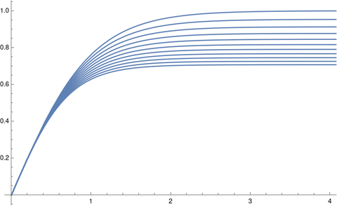
Think of m as a knob attached to the sn function. When we turn the knob to 0 we get the sine function. As we turn the knob up, sn becomes less like sine and more like hyperbolic tangent. The period becomes longer as a function of m, diverging to infinity as m approaches 1. Here’s a plot of one period of sn(x, m) for several values of m.

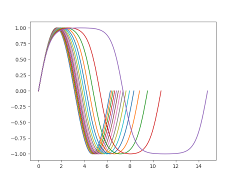
So while it’s true that sn can be thought of as a generalization of sine, it’s also a generalization of hyperbolic tangent.

Similarly, cn can be thought of as a generalization of cosine, but it’s also a generalization of hyperbolic secant.

All of the Jacobi functions are circular functions when m = 0 and hyperbolic functions when m = 1, with a caveat that we’ll get to shortly.

The extra function

For the rest of this article, I’d like to say there are seven circular functions, making the constant function 1 an honorary trig function. I’d also like to call it a hyperbolic function and a Jacobi function.

With this addition, we can say that the seven circular functions consist of {sin, cos, 1} and all their ratios. And the seven hyperbolic functions consist of {sinh, cosh, 1} and all their ratios.

The 13 Jacobi functions consist of {sn, cn, dn, 1} and all their ratios.

Circular functions are Jacobi functions

I mentioned above that sn(z, 0) = sin(z) and cn(z, 0) = cos(z). And the honorary Jacobi function 1 is always 1, regardless of m. So by taking ratios of sn, cn, and 1 we can obtain all ratios of sin, cos, and 1. Thus all circular functions correspond to a Jacobi function with m = 0.

There are more Jacobi functions than circular functions. We’ve shown that some Jacobi functions are circular functions when m = 0. Next we’ll show that all Jacobi functions are circular functions when m = 0.  For this we need one more fact:

dn(z. 0) = 1.

Never mind what dn is. For the purpose of this article it’s just one of the generators for the Jacobi functions. Since all the generators of the Jacobi functions are circular functions when m = 0, it follows that all Jacobi functions are circular functions when m = 0. Note that this would not be true if we hadn’t decided to call 1 a Jacobi function.

Hyperbolic functions are Jacobi functions

We can repeat the basic argument above to show that when m = 1, hyperbolic functions are Jacobi functions and Jacobi functions are hyperbolic functions.

I mentioned above that sn(z, 1) = tanh(z) and cn(z, 1) = sech(z). I said above that the hyperbolic functions are generated by {sinh, cosh, 1} but they are also generated by {tanh, sech, 1} because

cosh(z) = 1/sech(z)

and

sinh(z) = tanh(z) / sech(z).

A set of generators for the hyperbolic functions are Jacobi functions with m = 1, so all hyperbolic functions and Jacobi functions with m = 1. To prove the converse we also need the fact that

dn(z, 1) = sech(z).

Since sn, cn, dn, 1 correspond to hyperbolic functions when m = 1, all Jacobi functions do as well.

When Jacobi functions aren’t elliptic

The Jacobi functions are elliptic functions in general, but not when m = 0 or 1. So it’s not quite right to say that the circular and hyperbolic functions are special cases of the Jacobi elliptic functions. More precisely, they are special cases of the Jacobi functions, functions which are almost always elliptic, though not in the special cases discussed here. You might say that circular and hyperbolic functions are degenerate elliptic functions.

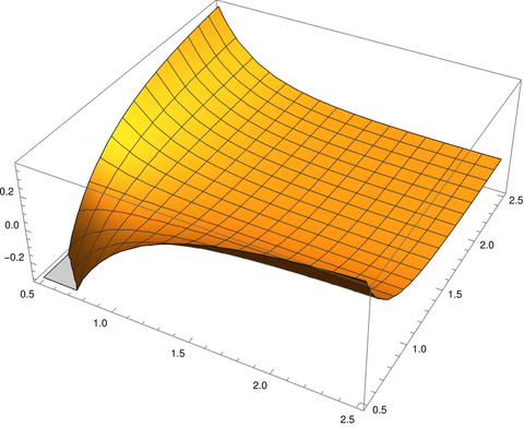
Elliptic functions are doubly periodic. They repeat themselves in two independent directions in the complex plane.

Circular functions are periodic along the real axis but not along the imaginary axis.

Hyperbolic functions are periodic along the imaginary axis but not along the real axis.

Jacobi functions have a horizontal period and a vertical period, and both are functions of m. When 0 < m < 1 both periods are finite. When m = 0 the vertical period becomes infinite, and when m = 1 the horizontal period becomes infinite.


What good is a DE once you have the solution?

In an undergraduate course on differential equations, you see an equation, you find a solution. Wax on, wax off. It would be reasonable to assume that the differential equation is simply an obstacle to overcome and that once you have the solution, the differential equation has done its job and can be discarded.

It would seem backward to ask whether a function satisfies a differential equation. It is backward, but that doesn’t mean it’s a bad idea. It can be very useful to know that a function you’re interested in satisfies a nice differential equation. (It’s trivial to make up differential equations for any function; the key is to discover a nice differential equation, a simple relationship between a function and its derivatives.)

The previous post gave an example of this. There we said that although Halley’s root-finding method converges faster than Newton’s method, it also requires one more function evaluation, namely the second derivative of the function whose root you’re finding. But when that function satisfies a second order differential equation, you can get the second derivative for free once you’ve evaluated the function and its derivative. Well, at a deep discount at least if not free.

In that post we gave the example of a Bessel function. Once you have evaluated a Bessel function and its first derivative at a point. you can calculate the second derivative in much less time that it took to evaluate the Bessel function itself.

Bessel functions are not unique in this regard. Hypergeometric functions are a large and useful class of functions, and these functions all satisfy Riemann’s differential equation.

All the classic orthogonal polynomials—Chebyshev polynomials, Jacobi polynomials, Laguerre polynomials, Hermite polynomials, etc.—satisfy a linear second order differential equation. For example, the Legendre polynomials Pn satisfy

(1 - x^2) y''(x) - 2 x y'(x) + \nu (\nu + 1) y = 0

And its not just Bessel functions, hypergeometric functions, and orthogonal polynomials. Most special functions satisfy a useful differential equation. More specifically, a linear second order differential equation.

So far the only reason given for wanting to know what differential equation a function satisfies is to speed up calculations: evaluate two functions and get a third one for cheap. But there are many other reasons to care what differential equation a function satisfies. For example, a common way to show that two functions are equal is to show that they satisfy the same differential equation with the same initial conditions. This is applying a uniqueness theorem for differential equations, but many other equations about differential equations could be useful to apply.

Related posts

Bounds on the incomplete beta function (beta CDF)

The incomplete beta function is defined by

B(x, y, z) = \int_0^z t^{x-1} (1-t)^{y-1} \, dx

It is called incomplete because the limit of integration doesn’t necessarily run all the way up to 1. When z = 1 the incomplete beta function is simply the beta function

B(x, y) = B(x, y, 1)

discussed in the previous post [1].

The incomplete beta function is proportional to the CDF of a beta random variable, and the proportionality constant is 1/B(x, y). That is, if X is a beta(a, b) random variable, then

\text{Prob}(X \leq x) = \frac{B(a, b, x)}{B(a, b)}

The right-hand side of the equation above is often called the regularized incomplete beta function. This is what an analyst would call it. A statistician would call it the beta distribution function.

The previous post gave simple bounds on the (complete) beta function. This post gives bounds on the incomplete beta function. These bounds are more complicated but also more useful. The incomplete beta function is more difficult to work with than the beta function, and so upper and lower bounds are more appreciated.

One application of these bounds would be to speed up software that evaluates beta probabilities. If you only need to know whether a probability is above or below some threshold, you could first compute an upper or lower bound. Maybe computing the exact probability is unnecessary because you can decide from your bounds whether the probability is above or below your threshold. If not, then you compute the exact probability. This is less work if your bounds are usually sufficient, and more work if they’re usually not. In the former case this could result in a significant speed up because the incomplete beta function is relatively expensive to evaluate.

Cerone, cited in the previous post, gives two lower bounds, L1 and L2, and two upper bounds, U1 and U2, for B(x, y, z). Therefore the maximum of L1 and L2 is a lower bound and the minimum of U1 and U2 is an upper bound. The bounds are complicated, but easier to work with than the incomplete beta function.

\begin{align*} L_1 &= \frac{z^{x-1}}{y} \left[ \left(1 - z + \frac{z}{x} \right)^y - (1-z)^y \right] \\ U_1 &= \frac{z^{x-1}}{y} \left[ 1 - \left(1 - \frac{z}{x}\right)^y\right] \\ L_2 &= \frac{\lambda(z)^x}{x} + (1-z)^{y-1}\, \frac{z^x - \lambda(z)^x}{x} \\ U_2 &= (1-z)^{y-1} \frac{\left( x - \lambda(z) \right)^x}{x} + \frac{z^x - \left(z - \lambda(z)\right)^x}{x} \\ \end{align*}

where

\lambda(z) = \frac{1 - (1-z)[1 - z(1-y)]}{y\left[1-(1-z)^{y-1}\right]}

Related posts

[1] Incidentally, Mathematica overloads the Beta function just as we overload B. Mathematica’s Beta[x, y] corresponds to our B(x, y), but the three-argument version of Beta, the incomplete beta function, puts the limit of integration z first. That is, our B(x, y, z) corresponds to Beta[z, x, y] in Mathematica.

Upper and lower bounds on the beta function

The beta function B(x, y) is defined by

B(x, y) = \int_0^1 t^{x-1} (1-t)^{y-1}\, dt

and is the normalizing constant for the beta probability distribution. It is related to the gamma function via

B(x, y) = \frac{\Gamma(x)\,\Gamma(y)}{\Gamma(x+y)}

The beta function comes up often in applications. It can be challenging to work with, however, and so estimates for the function are welcome.

The function 1/xy gives simple approximation and upper bound for B(x, y). Alzer [1] proved that when x > 1 and y > 1

0 \leq \frac{1}{xy} - B(x,y) \leq b

where the constant b is defined by

b = \max_{x\geq1}\left( \frac{1}{x^2} - \frac{\Gamma(x)^2}{\Gamma(2x)} \right) = 0.08731\ldots

Cerone [2] gives a different bound which varies with x and y and is usually better than Alzer’s bound. For x and y greater than 1, Cerone shows

0 \leq \frac{1}{xy} - B(x,y) \leq C(x) C(y) \leq b'

where

C(x) = \frac{x-1}{x\sqrt{2x-1}}

and

C(x) = \frac{x-1}{x\sqrt{2x-1}}

Cerone’s bound is slightly larger in the worst case, near x = y = (3 + √5)/2, but is smaller in general.

The difference between B(x, y) and 1/xy is largest when x or y is small. We can visualize this with the Mathematica command

    Plot3D[Beta[x, y] - 1/(x y), {x, 0.5, 2.5}, {y, 0.5, 2.5}]

which produces the following plot.

The plot dips down in the corner where x and y are near 0.5 and curls upward on the edges where one of the variables is near 0.5 and the other is not.

Let’s look at B(x, y) and 1/xy at along a diagonal slice (3t, 4t).

This suggests that approximating B(x, y) with 1/xy works best when the arguments are either small or large, with the maximum difference being when the arguments are moderate-sized. In the plot we see B(3, 4) is not particularly close to 1/12.

Next lets look at 1/xyB(x, y) along the same diagonal slice.

This shows that the error bound C(x) C(y) is not too tight, but better than the constant bound except near the maximum of 1/xyB(x, y).

Related posts

[1] H. Alzer. Monotonicity properties of the Hurwitz zeta function. Canadian Mathematical Bulletin 48 (2005), 333–339.

[2] P. Cerone. Special functions: approximations and bounds. Applicable Analysis and Discrete Mathematics, 2007, Vol. 1, No. 1, pp. 72–91

nth root of n!

Last week the function

b(n) = \exp\left(\frac{\log n!}{n} \right ) = \sqrt[n]{n!}

came up in a blog post as the solution to the equation n! = bn.

After writing that post I stumbled upon an article [1] that begins by saying, in my notation,

The function b(x) … has many applications in pure and applied mathematics.

The article mentions a couple applications but mostly focuses on approximations and bounds for the function b(x) and especially for the ratio b(x)/b(x + 1). In the article x is a positive real number, not necessarily an integer.

b(x) = \Gamma(x+1)^{1/x}

One of the results is the approximation

\frac{b(x)}{b(x+1)} \approx \left(\sqrt{2\pi x}\right)^{\frac{1}{x(x+1)}}

which is the beginning of an asymptotic series given in the paper.

Another result is the following upper and lower bounds on b(n).

\exp\left(-\frac{1}{2x}\right) < \left(1 + \frac{1}{x}\right)^x \frac{b(x)}{x \left(\sqrt{2\pi x}\right)^{1/x}} < \exp\left(-\frac{1}{2x} + \frac{5}{12x^2}\right)

Let’s look at some examples of these results using the following Python script.

    from numpy import exp, pi
    from scipy.special import loggamma
    
    b = lambda x: exp(loggamma(x+1)/x)
    
    bratio = lambda x: b(x)/b(x+1)
    
    bratio_approx = lambda x: (2*pi*x)**(0.5/(x*(x+1)))
    
    def lower_bound_b(x):
        r = exp(-0.5/x) * x*(2*pi*x)**(0.5/x)
        r /= (1 + 1/x)**x
        return r
    
    def upper_bound_b(x):
        return lower_bound_b(x)*exp(5/(12*x*x))
    
    for x in [25, 100, 1000]:
        print(bratio(x), bratio_approx(x))
    
    for x in [25, 100, 1000]:
        print(lower_bound_b(x), b(x), upper_bound_b(x))

The code exercising the ratio approximation prints

    0.964567 1.003897
    0.990366 1.000319
    0.999004 1.000004

and the code exercising the lower and upper bounds prints the following.

     10.170517  10.177141   10.177299
     37.991115  37.992689   38.992698
    369.491509 369.491663  369.491663

[1] Chao-Ping Chen and Cristinel Mortici. Asymptotic expansions and inequalities relating to the gamma function. Applicable Analysis and Discrete Mathematics, Vol. 16, No. 2 (October, 2022), pp. 379–399

Drag equation exponent variation

The motion of a falling body of mass m is given by

m \frac{dv}{dt} = mg - kv^r

where the term −kvr accounts for drag due to air resistance. One can derive r = 2 under simple physical assumptions, but if I remember correctly other values of r may be more realistic in certain circumstances. I don’t know much about the physics here; if you know about the use of other values of r, please let me know by leaving a comment.

Terminal velocity

When r = 1 or r = 2 the differential equation above can be solved in terms of elementary functions, but otherwise it cannot. Nevertheless one can show that for all values of r the object reaches a terminal velocity, and calculate that velocity without explicitly solving the differential equation. William Waterhouse demonstrated this in a one-page article [1]. He rewrites the equation to look at time as a function of velocity rather than velocity as a function of time

\frac{dt}{dv} = \frac{1}{g} \frac{1}{1 - (k/mg)v^r}

and concludes

t = \frac{1}{g} \int_0^v \frac{dv}{1 - (k/mg)v^r} + t_0

He notes that the integral diverges as v approaches

 \left(\frac{mg}{k}\right)^{1/r}

and so that is the terminal velocity, i.e. it takes an infinite amount of time to achieve this velocity. Waterhouse recommends this derivation as “a good example of deriving information about a problem without knowing an explicit solution.”

I would add that such an approach is the norm, not an exception. A closed-form solution to a differential equation in nice when you can get it, but usually not possible. And even when you can find a closed-form solution, you may be able to achieve your goal more directly by not using it.

Hypergeometric solution

I suspected the differential equation could be solved for general values of r using special functions, and that is the case. Mathematica was able to evaluate the integral for t as a function of v in terms of a hypergeometric function.

v \, _2F_1\left(1,\frac{1}{r};1+\frac{1}{r};\frac{g k v^r}{m}\right)

When I asked Mathematica to solve the differential equation directly, it said that the solution is the inverse function of the function above. Apparently Waterhouse and Mathematica agree that it is easier to think of t as a function of v rather than the original formulation.

The notation 2F1 indicates there are two upper parameters and one lower parameter. In our application, the upper parameters are 1 and 1/r, the lower parameter is 1 + 1/r, and the function is evaluated at gkvr/m. You can find a brief introduction to hypergeometric functions here. A hypergeometric function 2F1 has a singularity at 1, and so we could derive the terminal velocity from the explicit solution.

Mathematica implementation

Let c = gk/m. Then we can express velocity as a function of time in Mathematica by

    f[r_, c_, v_] := InverseFunction
    [
        #1 Hypergeometric2F1[1, 1/r, 1 + 1/r, c #1^r] &
    ][t]

and use this to make plots of the velocity for various values of c and r.

The following sets c = 2 and varies r over 1, 1.1, 1.2, … 2.

    Plot[Table[f[2, d/10, t], {d, 10, 20}], {t, 0, 4}, PlotRange -> All]

Here’s the output.

The terminal velocity decreases as r increases. The opposite is true for c < 1.

[1] William C. Waterhouse. A Fact about Falling Bodies. Mathematics Magazine, Vol. 44, No. 1 (Jan., 1971), pp. 33–34. The article straddles two pages, but takes up less than half of each page.

Every factorial is a power

The previous post mentioned that 24! ≈ 1024 and 25! ≈ 1025.

For every n, there is some base b such that n! = bn. For example, 30! ≈ 1230.

It’s easy to find b [1]:

b = \exp\left( \frac{\log n!}{n} \right)

What’s interesting is that b is very nearly a linear function of n.

In hindsight it’s clear that this should be the case—it follows easily from Stirling’s approximation—but I didn’t anticipate this before I plotted it.

Now fix n and find b such that n! = bn. Since the relationship between n and b(n) is nearly linear, this suggests

(2n)! \approx (2b)^{2n} = 2^{2n} (n!)^2

which is true. It follows from the multiplication identity for the gamma function:

Let z = n + 1/2 so that the left side is (2n)!. On the right side, Γ(z + 1/2) = n! and Γ(z) is not too different from n!. The rest of the right side is 22n/√π.

So our observation that b(n) is nearly linear gave us a hint of Gauss’s multiplication formula.

[1] Numerically you would probably evaluate this function by calling a routine that computes log Γ(n + 1) directly without computing Γ(n + 1) first. This avoids overflow for large n.

This is why mathematical libraries will have not only gamma functions but also loggamma functions. The latter seems redundant, but it’s not.

Maxwell-Boltzmann and Gamma

When I shared an image from the previous post on Twitter, someone who goes by the handle Nonetheless made the astute observation that image looked like the Maxwell-Boltzmann distribution. That made me wonder what 1/Γ(x) would be like turned into a probability distribution, and whether it would be approximately like the Maxwell-Boltzmann distribution.

(Here I’m looking at something related to what Nonetheless said, but different. He was looking at my plot of the error in approximating 1/Γ(x) by partial products, but I’m looking at 1/Γ(x) itself.)

Making probability distributions

You can make any non-negative function with a finite integral into a probability density function by dividing it by its integral. So we can define a probability density function

f(x) = \frac{c}{\Gamma(x)}

where

1/c = \int_0^\infty \frac{dx}{\Gamma(x)}

and so c = 0.356154. (The integral cannot be computed in closed form and so has to be evaluated numerically.)

Here’s a plot of f(x).

Note that we’re doing something kind of odd here. It’s common to see the gamma function in the definition of probability distributions, but the function is always evaluated at distribution parameters, not at the free variable x. We’ll give an example of this shortly.

Maxwell-Boltzmann distribution

The Maxwell-Boltzmann distribution, sometimes called just the Maxwell distribution, is used in statistical mechanics to give a density function for particle velocities. In statistical terminology, the Maxwell-Boltzmann distribution is a chi distribution [1] with three degrees of freedom and a scale parameter σ that depends on physical parameters.

The density function for a Maxwell-Boltzmann distribution with k degrees of freedom and scale parameter σ has the following equation.

\chi(x; k, \sigma) = \frac{1}{2^{(k/2) -1}\sigma \Gamma(k/2)} \left(\frac{x}{\sigma}\right)^{k-1} \exp(-x^2/2\sigma^2)

Think of this as xk-1 exp(-x² / 2σ²) multiplied by whatever you have to multiply it by to make it integrate to 1; most of the complexity in the definition is in the proportionality constant. And as mentioned above, the gamma function appears in the proportionality constant.

For the Maxwell-Boltzmann distribution, k = 3.

Lining up distributions

Now suppose we want to compare the distribution we’ve created out of 1/Γ(x) with the Maxwell-Boltzman distribution. One way of to do this would be to align the two distributions to have their peaks at the same place. The mode of a chi random variable with k degrees of freedom and scale σ is

x = \sqrt{k-1} \, \sigma

and so for a given k we can solve for σ to put the mode where we’d like.

For positive values, the minimum of the gamma function, and hence the maximum of its reciprocal, occurs at 1.46163. As with the integral above, this has to be computed numerically.

For the Maxwell-Boltzmann distribution, i.e. when k = 3, we don’t get a very good fit.

The tails on the chi distribution are too thin. If we try again with k = 2 we get a much better fit.

You get an even better fit with k = 1.86. The optimal value of k would depend on your criteria for optimality, but k = 1.86 looks like a good value just eyeballing it.

[1] This is a chi distribution, not the far more common chi-square distribution. The first time you see this is looks like a typo. If X is a random variable with a chi random variable with k degrees of freedom then X² has a chi-square distribution with k degrees of freedom.