Addition theorems

Posted on 6 October 2023 by John

Earlier this week I wrote about several ways to generalize trig functions. Since trig functions have addition theorems like

$\begin{align*} \sin(\theta \pm \varphi) &= \sin\theta \cos\varphi \pm \cos\theta \sin\varphi \\ \cos(\theta \pm \varphi) &= \cos\theta \cos\varphi \mp \sin\theta \sin\varphi \\ \tan(\theta \pm \varphi) &= \frac{\tan\theta \pm \tan\varphi}{1 \mp \tan\theta \tan\varphi} \end{align*}$

a natural question is whether generalized trig functions also have addition theorems.

Hyperbolic functions have well-known addition theorems analogous to the addition theorems above. This isn’t too surprising since circular and hyperbolic functions are fundamentally two sides of the same coin.

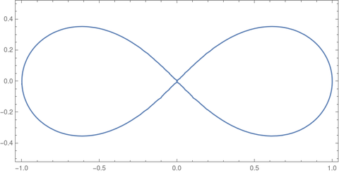
I mentioned that the lemniscate functions satisfy many identities but didn’t give any examples. Here are addition theorems satisfied by the lemniscate sine sl and the lemniscate cosine cl.

$\begin{aligned} \text{cl}\,(x+y) &= \frac{\text{cl}\,x\, \text{cl}\,y - \text{sl}\,x\, \text{sl}\,y} {1 + \text{sl}\,x\, \text{cl}\,x\, \text{sl}\,y\, \text{cl}\,y} \\ \text{sl}\,(x+y) &= \frac{\text{sl}\,x\, \text{cl}\,y + \text{cl}\,x\, \text{sl}\,y} {1 - \text{sl}\,x\, \text{cl}\,x\, \text{sl}\,y\, \text{cl}\,y} \end{aligned}$

Addition theorems for sin_p and friends are harder to come by. In [1] the authors say “no addition formula for sin_p is known to us” but they did come up with a double-argument theorem for a special case of sin_p,q:

$\sin_{4/3, 4}(2x) = \frac{2 \sin_{4/3, 4}(x)\, (\cos_{4/3, 4}(x))^{1/3}}{\left( 1 + 4(\sin_{4/3, 4}(x))^4 \,(\cos_{4/3, 4}(x))^{4/3} \right)^{1/2}}$

There is a deep reason why the lemniscate and hyperbolic functions have addition theorems and sin_p does not, namely a theorem of Weierstrass. This theorem says that a meromorphic function has an algebraic addition theorem if and only if it is an elliptic function of z, a rational function of z, or a rational function of exp(λz).

The leminscate functions have addition theorems because they are elliptic functions. Circular and hyperbolic functions have addition theorems because they are rational functions of exp(iz). But sin_p does not have an addition theorem because it is not elliptic, rational, or a rational function of exp(λz). It’s possible that sin_p has some sort of addition theorem that falls outside of Weiersrass’ theorem, i.e. an addition theorem using a non-algebraic function.

You may have noticed that the addition rule for sine involves not only sine but also cosine. But using the Pythagorean identity we can turn an addition rule involving sines and cosines into one only involving sines. Similarly, we can use a Pythagorean-like theorem to turn the identities involving sl and cl into identities involving only one of these functions.

Elliptic functions satisfy addition theorems, and functions satisfying addition theorems are elliptic (or the other two cases of Weierstrass’ theorem). Rational functions of x and rational functions of exp(λz) are easy to spot, so if you see an unfamiliar function that has an algebraic addition theorem, you know it’s an elliptic function. If you saw the addition theorems for sl and cl before knowing what these functions are, you could say to yourself that these are probably elliptic functions.

You may see other theorems called addition theorems. For example, the gamma function satisfies an addition theorem, although it is not elliptic or rational. But this is a restricted kind of addition theorem: it applies to x + 1 and not to general x + y. Also, the Bessel functions have addition theorems, but these theorems involve infinite sums; they are not algebraic addition theorems.

[1] David E. Edmunds, Petr Gurka, Jan Lang. Properties of generalized trigonometric functions. Journal of Approximation Theory 164 (2012) 47–56.

p-norm trig functions and “squigonometry”

Posted on 4 October 2023 by John

This is the fourth post in a series on generalizations of sine and cosine.

The first post looked at defining sine as the inverse of the inverse sine. The reason for this unusual approach is that the inverse sine is given in terms of an arc length and an integral. We can generalize sine by generalizing this arc length and/or generalizing the integral.

The first post mentioned that you could generalize the inverse sine by replacing “2” with “p” in an integral. Specifically, the function

$F_p(x) = \int_0^x (1 - |t|^p)^{-1/p} \,dt$

is the inverse sine when p = 2 and in general is the inverse of the function sin_p. Unfortunately, there two different ways to define sin_p. We next present a generalization that includes both definitions as special cases.

Edmunds, Gurka, and Lang [1] define the function

$F_{p,q}(x) = \int_0^x (1 - t^q)^{-1/p} \,dt$

and define sin_p,q to be its inverse.

The definition of sin_p at the top of the post corresponds to sin_p,q with p = q in the definition of Edmunds et al.

The other definition, and the one we’ll use for the rest of the post, corresponds to sin_r,s where s = p and r = (p − 1)/p.

This second definition sin_p has a geometric interpretation analogous to that in the previous post for hyperbolic functions [2]. That is, we start at (1, 0) and move clockwise along the p-norm circle until we sweep out an area of α/2. When we have swept out that much area, we are at the point (cos_p α, sin_p α).

When p = 4, the p-norm circle is also known as a “squircle,” and the p-norm sine and cosine analogs are sometimes placed under the heading “squigonometry.”

Previous posts in the series

[1] David E. Edmunds, Petr Gurka, Jan Lang. Properties of generalized trigonometric functions. Journal of Approximation Theory 164 (2012) 47–56.

[2] Chebolu et al. Trigonometric functions in the p-norm https://arxiv.org/abs/2109.14036

Lemniscate functions

Posted on 4 October 2023 by John

In the previous post I said that you could define the inverse sine as the function that gives the arc length along a circle, then define sine to be the inverse of the inverse sine. The purpose of such a backward definition is that it generalizes to other curves besides the circle. For example, it generalizes to the lemniscate, a curve studied by Bernoulli.

The leminiscate in rectangular coordinates satisfies

and in polar coordinates

$r^2 = \cos 2\theta$

The function arcsl(x), analogous to arcsin(x), is defined as the length of the arc along the leminiscate from the origin to the point (x, y). The length of the arc from (x, y) to the x-axis is arccl(x).

$\begin{align*} \mbox{arcsl}(x) &= \int_0^x \frac{dt}{\sqrt{1 - t^4}} \\ \mbox{arccl}(x) &= \int_x^1 \frac{dt}{\sqrt{1 - t^4}} \\ \end{align*}$

The lemniscate sine, sl, is the inverse of arcsl, and the lemniscate cosine, cl, is the inverse of arccl. These functions were first studied by Giulio Fagnano three centuries ago.

The lemniscate functions sl and cl are elliptic functions, and so they have a lot of nice properties and satisfy a lot of identities. See Wikipedia, for example. Update: see this follow up post on addition theorems.

Lemniscate constant

As mentioned in the previous post, generalizations of the sine and cosine functions have corresponding generalizations of π.

Just as the period of sine and cosine is 2π, the period of lemninscate sine and lemniscate cosine is 2ϖ.

The number ϖ is called the lemniscate constant. It is written with Unicode character U+03D6, GREEK SMALL LETTER OMEGA PI. The LaTeX command is \upvarpi.

The lemnmiscate constant ϖ is related to Gauss’ constant G by ϖ = πG.

The area of a squircle is √2 ϖ.

There is also a connection to the beta function: 2ϖ = B(1/4, 1/2).

Generalized trigonometry

Posted on 4 October 2023 by John

In a recent post I mentioned in passing that trigonometry can be generalized from functions associated with a circle to functions associated with other curves. This post will go into that a little further.

The equation of the unit circle is

and so in the first quadrant

$y = \sqrt{1 - x^2}$

The length of an arc from (1, 0) to (cos θ, sin θ) is θ. If we write the arc length as an integral we have

$\int_0^{\sin \theta} (1 -t^2)^{-1/2} \,dt = \theta$

and so

$F(x) = \int_0^x (1 - t^2)^{-1/2} \,dt$

is the inverse sine of x. Sine is the inverse of the inverse of sine, so we could define the sine function to be the inverse of F.

This would be a complicated way to define the sine function, but it suggests ways to create variations on sine: take the length of an arc along a curve other than the circle, and call the inverse of this function a new kind of sine. Or tinker with the integral defining F, whether or not the resulting integral corresponds to the length along a familiar curve, and use that to define a generalized sine.

Example: sin_p

We can replace the 2’s in the integral above with p‘s, defining F_p as

$F_p(x) = \int_0^x (1 - |t|^p)^{-1/p} \,dt$

and defining sin_p to be the inverse of F_p. When p = 2, sin_p(x) = sin(x). This idea goes back to E. Lungberg in 1879.

The function sin_p has its applications. For example, just as the sine function is an eigenfunction of the Laplacian, sin_p is an eigenfunction of the p-Laplacian.

We can extend sin_p to be a periodic function with period 4F_p(1). The constants π_p are defined as 2F_p(1) so that sin_p has period π_p and π₂ = π.

Future posts

I intend to explore several generalizations of sine and cosine. What happens if you replace a circle with an ellipse or a hyperbola? Or a squircle? How do these variations on sine and cosine compare to the originals? Do they satisfy analogous identities? How do they appear in applications? I’d like to address some of these questions in future posts.

Belt around an elliptical waist

Posted on 9 September 2023 by John

I just saw a tweet from Dave Richeson saying

I remember as a kid calculating the size difference (diameter) of a belt between each hole. Now I think about it every time I wear a belt.

Holes 1 inch apart change the diameter by about one-third of an inch (1/π). [Assuming people have a circular waistline 🤣]

People do not have circular waistlines, unless they are obese, but the circular approximation is fine for reasons we’ll show below.

Robust approximations

Good simplifications, such as approximating a human waist by a circle, are robust. It doesn’t matter how well a circle approximates a waistline but rather how well the conclusion assuming a circular waistline approximates the conclusion for a real waistline.

There’s a joke that physicists say things like “assume a spherical cow.” Obviously cows are not spherical, but depending on the context, assuming a spherical cow may be a very sensible thing to do.

Elliptical waistlines

A human waistline may be closer to an ellipse than a circle. It’s not an ellipse either—it varies from person to person—but my point here is to show that using a different model results in a similar conclusion.

For a circle, the perimeter equals π times the diameter. So an increase of 1 inch in the diameter corresponds to an increase of 1/π in the perimeter, as Dave said.

Suppose we increase the perimeter of an ellipse by 1 and keep the aspect ratio of the ellipse the same. How much do the major and minor axes change?

The answer will depend on the aspect ratio of the ellipse. I’m going to guess that the aspect ratio is maybe 2 to 1. This corresponds to eccentricity e equal to 0.87.

The ratio of the perimeter of an ellipse to its major axis is 2E(p) where E is the complete elliptic integral of the second kind. (See, there’s a good reason Dave used a circle rather than an ellipse!)

For a circle, the eccentricity is 0, and E(0) = π/2, so the ratio of perimeter to the major axis (i.e. diameter) is π. For eccentricity 0.87 this ratio is 2.42. So a change in belt size of 1 inch would correspond to a change in major axis of 0.41 and a change in minor axis of 0.21.

Dave’s estimate of 1/3 of an inch the average of these two values. If you average the major and minor axes of an ellipse and call that the “diameter” then Dave’s circular model comes to about the same conclusion as our elliptical model, but avoids having to use elliptic integrals.

Perimeter to average axis ratio

The following graph shows the ratio of perimeter to average axis length for an ellipse. On the left end, aspect 1, we have a circle and the ratio is π. As the aspect ratio goes to infinity, the limiting value is 4.

Even for substantial departures from a circle, such as a 2 : 1 or 3 : 1 aspect ratio, the ratio isn’t far from π.

Area and volume of hypersphere cap

Posted on 9 August 2023 by John

A spherical cap is the portion of a sphere above some horizontal plane. For example, the polar ice cap of the earth is the region above some latitude. I mentioned in this post that the area above a latitude φ is

$A = 2\pi R^2(1-\sin\varphi)$

where R is the earth’s radius. Latitude is the angle up from the equator. If we use the angle θ down from the pole, we get

$A = 2\pi R^2(1-\cos\theta)$

I recently ran across a generalization of this formula to higher-dimensional spheres in [1]. This paper uses the polar angle θ rather than latitude φ. Throughout this post we assume 0 ≤ θ ≤ π/2.

The paper also includes a formula for the volume of a hypersphere cap which I will include here.

Definitions

Let S be the surface of a ball in n-dimensional space and let A_n(R) be its surface area.

$A_n(R) = \frac{\pi^{n/2}}{\Gamma(n/2)} R^{n-1}$

Let I_x(a, b) be the incomplete beta function with parameters a and b evaluated at x. (This notation is arcane but standard.)

$I_x(a, b) = \int_0^x t^{a-1}\, (1-t)^{b-1}\, dt$

This is, aside from a normalizing constant, the CDF function of a beta(a, b) random variable. To make it into the CDF, divide by B(a, b), the (complete) beta function.

$B(a, b) = \int_0^1 t^{a-1}\, (1-t)^{b-1}\, dt$

Area equation

Now we can state the equation for the area of a spherical cap of a hypersphere in n dimensions.

$A_n^{\text{cap}}(R) = \frac{1}{2}A_n(R)\, I_{\sin^2\theta}\left(\frac{n-1}{2}, \frac{1}{2} \right )$

Recall that we assume the polar angle θ satisfies 0 ≤ θ ≤ π/2.

It’s not obvious that this reduces to the equation at the top of the post when n = 3, but it does.

Volume equation

The equation for the volume of the spherical cap is very similar:

$V_n^{\text{cap}}(R) = \frac{1}{2}V_n(R)\, I_{\sin^2\theta}\left(\frac{n+1}{2}, \frac{1}{2} \right )$

where V_n(R) is the volume of a ball of radius R in n dimensions.

$V_n(R) = \frac{\pi^{n/2}}{\Gamma\left(\frac{n}{2} + 1\right)} R^n$

[1] Shengqiao Li. Concise Formulas for the Area and Volume of a Hyperspherical Cap. Asian Journal of Mathematics and Statistics 4 (1): 66–70, 2011.

Extending harmonic numbers

Posted on 25 July 2023 by John

For a positive integer n, the nth harmonic number is defined to be the sum of the reciprocals of the first n positive integers:

$H_n = 1 + \frac{1}{2} + \frac{1}{3} + \cdots + \frac{1}{n}$

How might we extend this definition so that n does not have to be a positive integer?

First approach

One way to extend harmonic numbers is as follows. Start with the equation

$(t - 1)(t^{n-1} + t^{n-2} + t^{n-3} + \cdots + 1) = t^n - 1$

Then

$\frac{t^n - 1}{t-1} = t^{n-1} + t^{n-2} + t^{n-3} + \cdots + 1$

Integrate both sides from 0 to 1.

$\int_0^1\frac{t^n - 1}{t-1} \,dt = \frac{1}{n} + \frac{1}{n-1} + \frac{1}{n-2} + \cdots + 1 = H_n$

So when x is an integer,

$H_x = \int_0^1\frac{t^x - 1}{t-1} \,dt$

is a theorem. When x is not an integer, we take this as a definition.

Second approach

Another approach is to start with the identity

$\Gamma(x+1) = x\, \Gamma(x)$

then take the logarithm and derivative of both sides. This gives

$\psi(x+1) = \frac{1}{x} + \psi(x)$

where the digamma function ψ is defined to be the derivative of the log of the gamma function.

If x is an integer and we apply the identity above repeatedly we get

$\psi(n+1) = H_n + \psi(1) = H_n - \gamma$

where γ is Euler’s constant. Then we can define

$H_x = \psi(x + 1) + \gamma$

for general values of x.

Are they equal?

We’ve shown two ways of extending the harmonic numbers. Are these two different extensions or are they equal? They are in fact equal, which follows from equation 12.16 in Whittaker and Watson, citing a theorem of Legendre.

Taking either approach as our definition we could, for example, compute the πth harmonic number (1.87274) or even the ith harmonic number (0.671866 + 1.07667i).

An addition rule

The digamma function satisfies an addition rule

$\psi(2z) = \frac{1}{2} \left( \psi(z) + \psi\left(z + \frac{1}{2}\right)\right) + \log 2$

which can be proved by taking the logarithm and derivative of Gauss’s multiplication rule for the gamma function.

Let z = x + 1/2 and add γ to both sizes. This shows that harmonic numbers satisfy the addition rule

$H_{2x} = \frac{1}{2}\left( H_{x-1/2} + H_x \right) + \log 2$

When does a function have an addition theorem?

Posted on 14 July 2023 by John

Motivating examples

The addition theorem for cosine says that

$\cos(x + y) = \cos x \cos y - \sin x \sin y$

and the addition theorem for hyperbolic cosine is analogous, though with a sign change.

$\cosh(x + y) = \cosh x \cosh y + \sinh x \sinh y$

An addition theorem is a theorem that relates a function’s value at x + y to its values at x and at y. The squaring function satisfies a very simple addition theorem

and the Jacobi function sn satisfies a more complicated addition theorem.

$\text{sn}(x + y) = \frac{ \text{cn}(x)\, \text{cn}(y) - \text{sn}(x) \,\text{sn}(y) \,\text{dn}(x) \,\text{dn}(y) }{ 1 - m \, \text{sn}^2(x) \,\text{sn}^2(y) }$

Defining an algebraic addition theorem

Which functions have addition theorems? Before we can answer this question we need to be more precise about what an addition theorem is. We’ve said that an addition theorem for φ relates φ(x + y) to φ(x) and φ(y). But what exactly do we mean by “relate”? What counts as a relation?

Also, the examples above don’t exactly satisfy this definition. The addition law for cosines, for example, relates cos(x + y) to the values of cos(x) and cos(y) but also to sin(x) and sin(y). Somehow that feels OK because sine and cosine are related. But here again we’re talking about things being related without saying exactly what we mean.

Weierstrass (1815–1897) made the idea of an addition theorem precise and classified functions having addition theorems. A function satisfies an algebraic addition theorem if there is a polynomial F in three variables such that

$F(\varphi(x + y), \varphi(x), \varphi(y)) = 0$

For example, if φ(x) = x² then

$\varphi(x+y)^2 - \left(\varphi(x)^2 + 2\varphi(x)\varphi(y) + \varphi(y)^2 \right) = 0$

and so we could take F to be

Similarly, if φ(x) = cos x then

$\left(\varphi(x+ y) - \varphi(x) \varphi(y)\right)^2 - (1 - \varphi(x))^2 (1 - \varphi(y))^2 = 0$

and so we could take F to be

Classifying functions with algebraic addition theorems

Now for Weierstrass’ theorem. A meromorphic function φ(z) has an algebraic addition theorem if and only if it is an elliptic function of z, a rational function of z, or a rational function of exp(λz).

A meromorphic function is one that is analytic everywhere except at isolated singularities. To put it another way, we assume φ has a convergent power series everywhere in the complex plane except at isolated points.

The examples above illustrate all three cases of Weierstrass’ theorem. The function sn(z) is elliptic, the function z² is rational, and the functions cos(z) and cosh(z) are rational functions of exp(iz).

Other kinds of addition theorems

Algebraic addition theorems are not the only kind of addition theorems. For example, Bessel functions satisfy a different kind of addition theorem:

$J_n(x + y) = \sum_{k=-\infty}^\infty J_{n-k}(x) J_k(y)$

This theorem relates the value of a Bessel function at x + y to the values of other Bessel functions at x and at y, but it is not an algebraic addition theorem because the right hand side is an infinite sum and because the Bessel functions are not algebraically related to each other.

Circular, hyperbolic, and elliptic functions

Posted on 9 July 2023 by John

This post will explore how the trigonometric functions and the hyperbolic trigonometric functions relate to the Jacobi elliptic functions.

There are six circular functions: sin, cos, tan, sec, csc, and cot.

There are six hyperbolic functions: just stick an ‘h’ on the end of each of the circular functions.

There are an infinite number of elliptic functions, but we will focus on 12 elliptic functions, the Jacobi functions.

sn, sin, and tanh

The Jacobi functions have names like sn and cn that imply a relation to sine and cosine. This is both true and misleading.

Jacobi functions are functions of two variables, but we think of the second variable as a fixed parameter. So the function sn(z, m), for example, is a family of functions of z, with a parameter m. When that parameter is set to 0, sn coincides with sine, i.e.

sn(z, 0) = sin(z).

And for small values of m, sn(z, m) is a lot like sin(z). But when m = 1,

sn(z, 1) = tanh(z).

Think of m as a knob attached to the sn function. When we turn the knob to 0 we get the sine function. As we turn the knob up, sn becomes less like sine and more like hyperbolic tangent. The period becomes longer as a function of m, diverging to infinity as m approaches 1. Here’s a plot of one period of sn(x, m) for several values of m.

So while it’s true that sn can be thought of as a generalization of sine, it’s also a generalization of hyperbolic tangent.

Similarly, cn can be thought of as a generalization of cosine, but it’s also a generalization of hyperbolic secant.

All of the Jacobi functions are circular functions when m = 0 and hyperbolic functions when m = 1, with a caveat that we’ll get to shortly.

The extra function

For the rest of this article, I’d like to say there are seven circular functions, making the constant function 1 an honorary trig function. I’d also like to call it a hyperbolic function and a Jacobi function.

With this addition, we can say that the seven circular functions consist of {sin, cos, 1} and all their ratios. And the seven hyperbolic functions consist of {sinh, cosh, 1} and all their ratios.

The 13 Jacobi functions consist of {sn, cn, dn, 1} and all their ratios.

Circular functions are Jacobi functions

I mentioned above that sn(z, 0) = sin(z) and cn(z, 0) = cos(z). And the honorary Jacobi function 1 is always 1, regardless of m. So by taking ratios of sn, cn, and 1 we can obtain all ratios of sin, cos, and 1. Thus all circular functions correspond to a Jacobi function with m = 0.

There are more Jacobi functions than circular functions. We’ve shown that some Jacobi functions are circular functions when m = 0. Next we’ll show that all Jacobi functions are circular functions when m = 0. For this we need one more fact:

dn(z. 0) = 1.

Never mind what dn is. For the purpose of this article it’s just one of the generators for the Jacobi functions. Since all the generators of the Jacobi functions are circular functions when m = 0, it follows that all Jacobi functions are circular functions when m = 0. Note that this would not be true if we hadn’t decided to call 1 a Jacobi function.

Hyperbolic functions are Jacobi functions

We can repeat the basic argument above to show that when m = 1, hyperbolic functions are Jacobi functions and Jacobi functions are hyperbolic functions.

I mentioned above that sn(z, 1) = tanh(z) and cn(z, 1) = sech(z). I said above that the hyperbolic functions are generated by {sinh, cosh, 1} but they are also generated by {tanh, sech, 1} because

cosh(z) = 1/sech(z)

and

sinh(z) = tanh(z) / sech(z).

A set of generators for the hyperbolic functions are Jacobi functions with m = 1, so all hyperbolic functions and Jacobi functions with m = 1. To prove the converse we also need the fact that

dn(z, 1) = sech(z).

Since sn, cn, dn, 1 correspond to hyperbolic functions when m = 1, all Jacobi functions do as well.

When Jacobi functions aren’t elliptic

The Jacobi functions are elliptic functions in general, but not when m = 0 or 1. So it’s not quite right to say that the circular and hyperbolic functions are special cases of the Jacobi elliptic functions. More precisely, they are special cases of the Jacobi functions, functions which are almost always elliptic, though not in the special cases discussed here. You might say that circular and hyperbolic functions are degenerate elliptic functions.

Elliptic functions are doubly periodic. They repeat themselves in two independent directions in the complex plane.

Circular functions are periodic along the real axis but not along the imaginary axis.

Hyperbolic functions are periodic along the imaginary axis but not along the real axis.

Jacobi functions have a horizontal period and a vertical period, and both are functions of m. When 0 < m < 1 both periods are finite. When m = 0 the vertical period becomes infinite, and when m = 1 the horizontal period becomes infinite.

What good is a DE once you have the solution?

Posted on 4 July 2023 by John

In an undergraduate course on differential equations, you see an equation, you find a solution. Wax on, wax off. It would be reasonable to assume that the differential equation is simply an obstacle to overcome and that once you have the solution, the differential equation has done its job and can be discarded.

It would seem backward to ask whether a function satisfies a differential equation. It is backward, but that doesn’t mean it’s a bad idea. It can be very useful to know that a function you’re interested in satisfies a nice differential equation. (It’s trivial to make up differential equations for any function; the key is to discover a nice differential equation, a simple relationship between a function and its derivatives.)

The previous post gave an example of this. There we said that although Halley’s root-finding method converges faster than Newton’s method, it also requires one more function evaluation, namely the second derivative of the function whose root you’re finding. But when that function satisfies a second order differential equation, you can get the second derivative for free once you’ve evaluated the function and its derivative. Well, at a deep discount at least if not free.

In that post we gave the example of a Bessel function. Once you have evaluated a Bessel function and its first derivative at a point. you can calculate the second derivative in much less time that it took to evaluate the Bessel function itself.

Bessel functions are not unique in this regard. Hypergeometric functions are a large and useful class of functions, and these functions all satisfy Riemann’s differential equation.

All the classic orthogonal polynomials—Chebyshev polynomials, Jacobi polynomials, Laguerre polynomials, Hermite polynomials, etc.—satisfy a linear second order differential equation. For example, the Legendre polynomials P_n satisfy

$(1 - x^2) y''(x) - 2 x y'(x) + \nu (\nu + 1) y = 0$

And its not just Bessel functions, hypergeometric functions, and orthogonal polynomials. Most special functions satisfy a useful differential equation. More specifically, a linear second order differential equation.

So far the only reason given for wanting to know what differential equation a function satisfies is to speed up calculations: evaluate two functions and get a third one for cheap. But there are many other reasons to care what differential equation a function satisfies. For example, a common way to show that two functions are equal is to show that they satisfy the same differential equation with the same initial conditions. This is applying a uniqueness theorem for differential equations, but many other equations about differential equations could be useful to apply.

Special functions

Addition theorems

p-norm trig functions and “squigonometry”

Previous posts in the series

Lemniscate functions

Lemniscate constant

Generalized trigonometry

Example: sin_p

Future posts

Belt around an elliptical waist

Robust approximations

Elliptical waistlines

Perimeter to average axis ratio

Related posts

Area and volume of hypersphere cap

Definitions

Area equation

Volume equation

Related posts

Extending harmonic numbers

First approach

Second approach

Are they equal?

An addition rule

Related posts

When does a function have an addition theorem?

Motivating examples

Defining an algebraic addition theorem

Classifying functions with algebraic addition theorems

Other kinds of addition theorems

Related posts

Circular, hyperbolic, and elliptic functions

sn, sin, and tanh

The extra function

Circular functions are Jacobi functions

Hyperbolic functions are Jacobi functions

When Jacobi functions aren’t elliptic

What good is a DE once you have the solution?

Related posts

Previous posts in the series

Lemniscate constant

Example: sinp

Future posts

Robust approximations

Elliptical waistlines

Perimeter to average axis ratio

Related posts

Definitions

Area equation

Volume equation

Related posts

First approach

Second approach

Are they equal?

An addition rule

Related posts

Motivating examples

Defining an algebraic addition theorem

Classifying functions with algebraic addition theorems

Other kinds of addition theorems

Related posts

sn, sin, and tanh

The extra function

Circular functions are Jacobi functions

Hyperbolic functions are Jacobi functions

When Jacobi functions aren’t elliptic

Related posts

Example: sin_p