A pragmatist takes the witness stand

The idea for my previous post was the following quote from Josias Royce responding to William James. James embraced philosophical pragmatism, the view that whatever is expedient is true.

Would you then get on the witness stand in a court of law and swear to tell ‘the expedient, the whole expedient and nothing but the expedient, so help me future experience’…?

Philosophical pragmatism is not simply pragmatism in the sense of valuing the practical. Instead it is the idea that the only test of truth is what works. But “works” by what criteria? Pragmatism is inadequate as a philosophical foundation because you need other criteria to decide what it means for something to “work.”

A relativist takes the witness stand

Here’s how a relativist would administer a judicial oath.

Do you solemnly swear to tell what’s true for you, the whole of what’s true for you, and only what’s true for you?

Would that make you feel a little uneasy if the person being sworn in were testifying against you? Assuming you’re innocent, wouldn’t you rather they just swear to tell the truth?

Update: See further discussion in A pragmatist takes the witness stand.

When the normal approximation for Student t isn’t good enough

Folk wisdom says that for all practical purposes, a Student-t distribution with 30 or more degrees of freedom is a normal distribution. Well, not for all practical purposes.

For 30 or more degrees of freedom, the error in approximating the PDF or CDF of a Student-t distribution with a normal is less than 0.005. So for many applications, the n > 30 rule of thumb is appropriate. (See these notes for details.)

However, sometimes you need to look at the quantiles of a t distribution, such as when finding confidence intervals. For example, when computing confidence intervals, you don’t need to evaluate the CDF of a Student-t distribution per se but rather the inverse of such a CDF. And in that case, the error in the normal approximation may be larger than you’d expect.

Say you’re computing a 95% confidence interval for the mean of a set of 31 data points. You first find t* such that P(t > t*) = 0.025 where t is a Student-t random variable with 31 – 1 = 30 degrees of freedom. Your confidence interval is the sample mean +/- t* s/√n where s is the sample standard deviation. For 30 degrees of freedom, t* = 2.04. If you used the normal approximation, you’d get 1.96 instead of 2.04, a relative error of about 4% meaning the error in computing your confidence interval is about 4%. While the error in normal approximation to the CDF is less than 0.005 for n > 30, the error in the normal approximation to the CDF inverse is an order of magnitude greater. Also, the error increases as the confidence increases. For example, for a 99% confidence interval, the error is about 6.3%.

It may be that none of this is a problem. If you only have 31 data points, there’s a fair amount of uncertainty in your estimate of the mean, and there’s no point in quantifying with great precision an estimate of how uncertain you are! Modeling assumptions are probably a larger source of error than the normal approximation to the Student-t.  But as a numerical problem, it’s interesting that the approximation error may be larger than expected. For n = 300, the error in the normal approximation to t* is about 0.4%. This means the error in the normal approximation to the inverse CDF is as good at n=300 as the normal approximation to the CDF itself is at n=30.

Errors in math papers not a big deal?

Daniel Lemire wrote a blog post this morning that ties together a couple themes previously discussed here.

Most published math papers contain errors, and yet there have been surprisingly few “major screw-ups” as defined by Mark Dominus. Daniel Lemire’s post quotes Doron Zeilberger on why these frequent errors are often benign.

Most mathematical papers are leaves in the web of knowledge, that no one reads, or will ever use to prove something else. The results that are used again and again are mostly lemmas, that while a priori non-trivial, once known, their proof is transparent. (Zeilberger’s Opinion 91)

Those papers that are “branches” rather than “leaves” receive more scrutiny and are more likely to be correct.

Zeilberger says lemmas get reused more than theorems. This dovetails with Mandelbrot’s observation mentioned a few weeks ago.

Many creative minds overrate their most baroque works, and underrate the simple ones. When history reverses such judgments, prolific writers come to be best remembered as authors of “lemmas,” of propositions they had felt “too simple” in themselves and had to be published solely as preludes to forgotten theorems.

There are obvious analogies to software.  Software that many people use has fewer bugs than software that few people use, just as theorems that people build on have fewer bugs than “leaves in the web of knowledge.” Useful subroutines and libraries are more likely to be reused than complete programs. And as Donald Knuth pointed out, re-editable code is better than black-box reusable code.

Everybody knows that software has bugs, but not everyone realizes how buggy theorems are. Bugs in software are more obvious because paper doesn’t abort. Proofs and programs are complementary forms of validation. Attempting to prove the correctness of an algorithm certainly reduces the chances of a bug, but proofs are fallible as well. Again quoting Knuth, he once said “Beware of bugs in the above code; I have only proved it correct, not tried it.” Not only can programs benefit from being more proof-like, proofs can benefit from being more program-like.

Upper and lower bounds on binomial coefficients

Binomial coefficients are easy to motivate and define. In its simplest form, the binomial coefficient (n, k) is the number of ways to choose k things from a set of n things and equals n!/(k! (nk)!). On the other hand, binomial coefficients can be hard to work with when proving theorems.

In applications, such as establishing bounds on an algorithm’s run time, it’s often enough to have upper bound or lower bounds on binomial coefficients that are easier to work with. Here’s a pair of such bounds.

\left( \frac{n}{k} \right)^k \leq {n \choose k} \leq \left( \frac{en}{k} \right)^k

for positive integers n and k with 1 ≤ kn.

The bounds above are easy to remember due to the typographical similarity between the three terms. Start with the binomial coefficient symbol. To get a lower bound, add a horizontal bar to turn the coefficient into a fraction and add an exponent of k. To get an upper bound, insert a factor of “e” inside the lower bound.

I found the bounds above in Introduction to Algorithms. The statement and proof were limited to integer arguments, but binomial coefficients can be defined more generally and the bounds appear to be valid for real values of n and k, not just integer values.

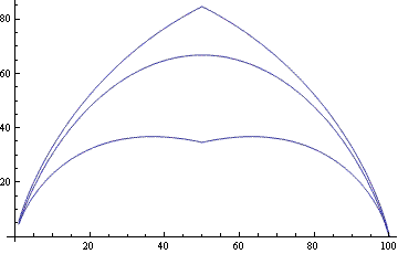
How good are the bounds? Here’s a plot of the upper and lower bounds as well as the true value. Because binomial coefficients can get very large, I plotted the logarithms of the bounds and true values. In this plot n = 100 and k varies between 1 and 100 (including non-integer values).
plotting log of binomial coefficients and bounds

The lower bound is exact at the left end and the right end and is worse in the middle.

The upper bound is quite good for small k but terrible for large k. However, we could easily improve the upper bound by using the fact that binomial(n, k) = binomial(n, nk). For k larger than n/2, we could apply the upper bound to nk rather than k. We could do the same for the lower bound, though the benefit in doing so is not as great.

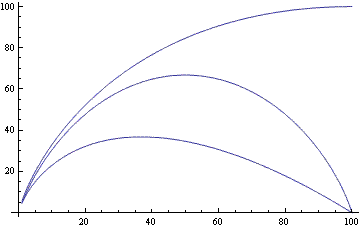
Here’s the plot that uses the best upper and lower bounds switching from binomial(n, k) to binomial(nk) for k > n/2.

plotting log of binomial coefficients using the better of k or n-k in the bounds

I experimented briefly with other values of n and got very similar plots.

Related post: How to compute binomial coefficients

Inside Steve Jobs’ brain

Last week I read Inside Drucker’s Brain and this week I’m reading Inside Steve’s Brain. The two books are written by different authors about very different men. But one theme that both books have in common is an appreciation for killing projects, even moderately successful projects, in order to focus on even more important projects.

So far, the thing I’ve found most impressive is how Steve Jobs dramatically reduced Apple’s product offerings in his plan to turn around the company.

When Jobs took over, Apple sold about forty different products … The lineup of computers was particularly baffling. There were several major lines … each with a dozen different models. But there was little to distinguish between the models except for their confusing product names.

The book goes on to describe Steve Job’s response.

Jobs drew a very simple two-by-two grid on the whiteboard. Across the top he wrote “Consumer” and “Professional,” and down the side, “Portable” and “Desktop.” Here was Apple’s new product strategy. Just four machines …

Sometimes I feel like I need to do something like that in my personal life, cutting my number of projects down by an order of magnitude.

I’m curious what the rest of the book holds. As I write this, most of the book’s reviews on Amazon are positive, four stars out of five on average. There’s only a single one-star review, but it’s worth considering. In a nutshell, the critic says the book is poorly written and contains little new material. He may be right. I’ll grant that the book isn’t the best prose I’ve ever read. But it doesn’t matter to me whether it’s original; I don’t know much about Steve Jobs, so the book’s content is new to me.