Inverse Gray code

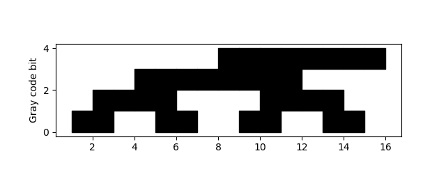
The previous post looked at Gray code, a way of encoding digits so that the encodings of consecutive integers differ in only bit. This post will look at how to compute the inverse of Gray code.

The Gray code of a non-negative integer n is given by

    def gray(n):
        return n ^ (n >> 1)

Bit-level operations

In case you’re not familiar with the notation, the >> operator shifts the bits of its argument. The code above shifts the bits of n one place to the right. In the process, the least significant bit falls off the end. We could replace n >> 1 with n // 2 if we like, i.e. integer division by 2, rounding down if n is odd. The ^ operator stands for XOR, exclusive OR. A bit of x ^ y is 0 if both corresponding bits in x and y are the same, and 1 if they are different.

Computing the inverse

The inverse of Gray code is a more complicated. If we assume n < 232, then we can compute the inverse Gray code of n by

    def inverse_gray32(n):
        assert(0 <= n < 2**32) n = n ^ (n >> 1)
        n = n ^ (n >> 2)
        n = n ^ (n >> 4)
        n = n ^ (n >> 8)
        n = n ^ (n >> 16)
        return n

For n of any size, we can compute its inverse Gray code by

    def inverse_gray(n):
        x = n
        e = 1
        while x:
            x = n >> e
            e *= 2
            n = n ^ x
        return n

If n is a 32-bit integer, inverse_gray32 is potentially faster than inverse_gray because of the loop unrolling.
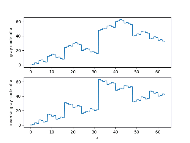
Plots

Here’s a plot of the Gray code function and its inverse.

Proof via linear algebra

How do we know that what we’re calling the inverse Gray code really is the inverse? Here’s a proof for 32-bit integers n.

    def test_inverse32():
        for i in range(32):
            x = 2**i
            assert(inverse_gray32(gray(x)) == x)
            assert(gray(inverse_gray32(x)) == x)

How is that a proof? Wouldn’t you need to try all possible 32-bit integers if you wanted a proof by brute force?

If we think of 32-bit numbers as vectors in a 32-dimensional vector space over the binary field, addition is defined by XOR. So XOR is linear by definition. It’s easy to see that shifts are also linear, and the composition of linear functions is linear. This means that gray and inverse_gray32 are linear transformations. If the two linear transformations are inverses of each other on the elements of a basis, they are inverses everywhere. The unit basis vectors in our vector space are simply the powers of 2.

Matrix representation

Because Gray code and its inverse are linear transformations, they can be defined by matrix multiplication (over the binary field). So we could come up with 32 × 32 binary matrices for Gray code and its inverse. Matrix multiplication would give us a possible, but inefficient, way to implement these functions. Alternatively, you could think of the code above as clever ways to implement multiplication by special matrices very efficiently!

OK, so what are the matrices? For n-bit numbers, the matrix giving the Gray code transformation has dimension n by n. It has 1’s on the main diagonal, and on the diagonal just below the main diagonal, and 0s everywhere else. The inverse of this matrix, the matrix for the inverse Gray code transformation, has 1s on the main diagonal and everywhere below.

Here are the matrices for n = 4.

\begin{bmatrix} 1 & 0 & 0 & 0 \\ 1 & 1 & 0 & 0 \\ 0 & 1 & 1 & 0 \\ 0 & 0 & 1 & 1 \\ \end{bmatrix} \begin{bmatrix} 1 & 0 & 0 & 0 \\ 1 & 1 & 0 & 0 \\ 1 & 1 & 1 & 0 \\ 1 & 1 & 1 & 1 \\ \end{bmatrix} = \begin{bmatrix} 1 & 0 & 0 & 0 \\ 0 & 1 & 0 & 0 \\ 0 & 0 & 1 & 0 \\ 0 & 0 & 0 & 1 \\ \end{bmatrix}

The matrix on the left is for Gray code, the next matrix is for inverse Gray code, and the last matrix is the identity. NB: The equation above only holds when you’re working over the binary field, i.e. addition is carried out mod 2, so 1 + 1 = 0.

To transform a number, represent it as a vector of length n, with the least significant in the first component, and multiply by the appropriate matrix.

Relation to popcount

It’s easy to see by induction that a number is odd if and only if its Gray code has an odd number of 1. The number 1 is its own Gray code, and as we move from the Gray code of n to the Gray code of n+1 we change one bit, so we change the parity of the the number of 1s.

There’s a standard C function popcount that counts the number of 1’s in a number’s binary representation, and the last bit of the popcount is the parity of the number of 1s. I blogged about this before here. If you look at the code at the bottom of that post, you’ll see that it’s the same as gray_inverse32.

The code in that post works because you can compute whether a word has an odd or even number of 1s by testing whether it is the Gray code of an odd or even number.

Gray code

Suppose you want to list the numbers from 0 to N in such a way that only one bit at a time changes between consecutive numbers. It’s not clear that this is even possible, but in fact it’s easy using Gray code, a method named after Frank Gray.

To convert an integer to its Gray code, take the XOR of the number with the number shifted right by 1.

    def gray(n): return n ^ n >> 1

Here’s a little Python code to demonstrate this.

    for i in range(8): print(format(gray(i), '03b'))

produces

    000
    001
    011
    010
    110
    111
    101
    100

Note that the numbers from 0 to 7 appear once, and each differs in exactly one bit from the numbers immediately above and below.

Let’s visualize the bits in Gray code with black squares for 1s and white squares for 0s.

The code that produced the plot is very brief.

    N = 4
    M = 2**N
    for i in range(N):
        for j in range(M):
            if gray(j) & 1<<i: # ith bit set
                plt.fill_between([j, j+1], i, i+1, color="k")
    plt.axes().set_aspect(1)
    plt.ylabel("Gray code bit")

The bits are numbered from least significant to most significant, starting with 1.

If you want to see the sequence carried out further, increase N. If you do, you may want to comment out the line that sets the aspect ratio to be square because otherwise your plot will be much longer than tall.

Note that the Gray code of 2n  − 1 is 2n−1, i.e. it only has one bit set. So if you were to wrap the sequence around, making a cylinder, you’d only change one bit at a time while going around the cylinder.

This could make a simple classroom activity. Students could reproduce the plot above by filling in squares on graph paper, then cut out the rectangle and tape the ends together.

See the next post for how to compute the inverse Gray code.

Related posts

Memorizing numbers and enumerating possibilities

This post will illustrate two things: how to memorize numbers, and how to enumerate products of sets in Python.

Major system

There’s a way of memorizing numbers by converting digits to consonant sounds, then adding vowels to make memorable words. It’s called the “major” mnemonic system, though it’s not certain where the system or the name came from.

I learned the major system as a child, but never used it. I thought about it more recently when I ran across the article Harry Potter and the Mnemonic Major System by Kris Fris.

Here is the encoding system in the form of a Python dictionary, using IPA symbols for the consonant sounds.

    digit_encodings = {
        0: ['s', 'z'],
        1: ['t', 'd', 'ð', 'θ'],
        2: ['n', 'ŋ'],
        3: ['m'],
        4: ['r'],
        5: ['l'],
        6: ['ʤ', 'ʧ', 'ʃ', 'ʒ'],
        7: ['k', 'g'],
        8: ['f', 'v'],
        9: ['p', 'b']
    }

The method is based on consonant sounds, not spelling. For example, the word “circle” would be a possible encoding of the number 0475. Note that the soft ‘c’ in circle encodes a 0 and the hard ‘c’ encodes a 7.

It’s curious that some digits have only one associated consonant sound, while others have up to four. The method was not originally designed for English, at least not modern English, and there may be some historical vestiges of other languages in the system. Even so, the sounds are fairly evenly spread out phonetically. It may not be optimal for English speakers, but some care went into designing it.

For more on the major system, see its Wikipedia page.

Enumerating set products

There are multiple consonant sound choices for a given digit, and so it would be natural to enumerate the possibilities when searching for a suitable encoding of a number.

If you only ever worked with two digit numbers, you could use a pair of for loops. But then if you wanted to work with three digit numbers, you’d need three nested for loops. For a fixed number of digits, this is messy, and for a variable number of digits it’s unworkable.

The function product from itertools gives an elegant solution. Pass in any number of iterable objects, and it will enumerate their Cartesian product.

    from itertools import product

    def enumerate_ipa(number):
        encodings = [digit_encodings[int(d)] for d in str(number)]
        for p in product(*encodings):
            print("".join(p))

In the code above, encodings is a list of lists of phonetic symbols. Unfortunately product takes lists as its argument, not a list of lists. The * operator takes care of unpacking encodings into the form product wants.

Example

Suppose you wanted to use the major system to memorize

1/π = .31830988

I’m not recommending that you memorize this number, or that you use the major system if you do want to memorize it, but let’s suppose that’s what you’d like to do.

You could break the digits into groups however you like, but here’s what you get if you divide them into 318, 309, and 88.

The digits in 318 could be encoded as mtf, mtv, mdf, mdv, mðf, mðv, mθf, or mθv.

The digits in 309 could be encoded as msp, msb, mzp, or mzb.

The digits in 88 could be encoded as ff, fv, vf, or vv.

So one possibility would be to encode 31830988 as “midwife mishap fife.” You could think of a pie that got turned upside down. It was the midwife’s mishap, knocked over while she was playing a fife.

Notice that the “w” sound in “midwife” doesn’t encode anything, nor does the “h” sound in “mishap.”

Related posts

Looking at the bits of a Unicode (UTF-8) text file

Suppose you type a little text into a text file, say “123”. If you open this file in a hex editor you’ll see

    3132 33

because the ASCII value for the character ‘1’ is 0x31 in hex, ‘2’ corresponds to 0x32, and ‘3’ corresponds to 0x33. If your file is saved as utf-8 rather than ASCII, it makes absolutely no difference, as long as the file is UTF-8 encoded. By design, UTF-8 is backward compatible with the first 128 ASCII characters.

Next, let’s add some Greek letters. Now our file contains “123 αβγ”. The lower-case Greek alphabet starts at 0x03B1, so these three characters are 0x03B1, 0x03B2, and 0x03B3. Now let’s look at the file in our hex editor.

    3132 3320 CEB1 CEB2 CEB3

The B1, B2, and B3 look familiar, but why do they have “CE” in front rather than “03”? This has to do with the details of UTF-8 encoding. If we looked at the same file with UTF-16 encoding, representing each character with 16 bits, the results look more familiar.

    FEFF 0031 0032 0033 0020 03B1 03B2 03B3

So our ASCII characters—1, 2, 3, and space—are padded with a couple zeros, and we see the Unicode values of our Greek letters as we expect. But what’s the FEFF at the beginning? That’s a byte order mark (BOM) that my text editor inserted. This is an invisible marker saying that the bytes are stored in big-endian mode.

Going back to UTF-8, the ASCII characters are more compact, i.e. no zero padding, but why to the Greek letters start with “CE”?

    3132 3320 CEB1 CEB2 CEB3

As I go into detail here, UTF-8 is a clever way to save space when representing mostly ASCII text. Since ASCII bytes start with 0, a byte starting with 1 signals that something special is happening and that the following bytes are to be interpreted differently.

In binary, 0xCE expands to

    11001110

I’ll color-code the bits to make it easier to talk about them.

    1 1 0 01110

The first 1 says that this byte does not simply represent a single character but is part of the encoding of a sequence of bytes encoding a character. The first 1 and the first 0, colored red, are bookends. The number of 1s in between, colored blue, says how many of the next bytes are part of this character. The bits after the first 0, colored black, are part of the character, and the rest follow in the next byte.

The continuation bytes begin with 10, and the remaining six bits are parts of a character. You know they’re not the start of a new character because there are no 1s between the first 1 and the first 0. With UTF-8, you can look at a byte in isolation and know whether it is an ASCII character, the beginning of a non-ASCII character, or the continuation of a non-ASCII character.

So now let’s look at 0xCEB1, with some spaces and colors added.

    1 1 0 01110 10 110001

The black bits, 01110110001, are the bits of our character, and the binary number 1110110001 is 0x03B1 in hex. So we get the Unicode value for α. Similarly the rest of the bytes encode β and γ.

It was a coincidence that the last two hex characters of our Greek letters were recognizable in the hex dump of the UTF-8 encoding. We’ll always see the last hex character of the Unicode value in the hex dump, but not always the last two.

For another example, let’s look at a higher Unicode value, U+FB31. This is בּ, the Hebrew letter bet with a dot in the middle. This shows up in a hex editor as

    EFAC B1

or in binary as

    111011111010110010110001

Let’s break this up as before.

    1 11 0 1111 10 101100 10 110001

The first bit is a 1, so we know we have some decoding to do. There are two 1s, colored blue, between the first 1 and the first 0, colored red. This says that the bits for our character, colored black, are stored in the remainder of the first byte and in the following two bytes.

So the bits of our character are

    1111101100110001

which in hex is 0xFB31, the Unicode value of our character.

More Unicode posts

How much do you really use?

I’ve been doing a little introspection lately about what software I use, not at an application level but at a feature level.

LaTeX

It started with looking at what parts of LaTeX I use. I wrote about this in April, and I revisited it this week in response to some client work [1]. LaTeX is second nature for me, so I figure that by now I’ve used a lot of its features.

Except I haven’t. When I searched my hard disk I found I’ve used a few hundred commands and a couple dozen packages. I’m fluent in LaTeX after using it for most of my life, but I don’t know it exhaustively. Far from it. Also, Pareto stuck his head in yet again: the 20% of commands I use most often account for about 80% of commands in my files.

Python

So next I started looking at what parts of Python I use by searching for import statements. I make heavy use of the usual suspects for applied math — numpy, scipy, sympy, matplotlib, etc. — but other than those I don’t use a lot of packages.

I was a little surprised to see that collections and functools are the non-mathematical packages I’ve used the most. A lot of the packages I’ve used have been hapax legomena, specialized packages I use one time.

Other tools

I imagine I’d get similar results if I looked at what parts of other programming languages and applications I use often. And for things I use less often, the percentage of features I use must be tiny.

When I needed to learn SQL, I took at look at the language standard. There were a bazillion statements defined in the standard, of which I may have used 10 by now. I imagine there are database gurus who haven’t used more than a few dozen statements.

Encouragement

I find all this encouraging because it means the next big, intimidating thing I need to learn probably won’t be that big in practice.

If you need to learn a new programming language and see that the “nutshell” book on the language is 1,500 pages, don’t be discouraged. The part you need to know may be fragments that amount to 30 pages, though it’s impossible to know in advance which 30 pages they will be.

Related posts

[1] I have a client that does a lot with org-mode. Rather than writing LaTeX files directly, they write org-mode files and export them to LaTeX. Although you can use LaTeX generously inside org-mode, you do have to do a few things a little differently. But it has its advantages.

  • Org has lighter markup and is easier to read.
  • You can run code inside an org file and have the source and/or the results inserted into the document.
  • Org cleans up after itself, deleting .aux files etc.
  • Org will automatically rerun the LaTeX compiler if necessary to get cross references right.
  • The outline features in org give you code folding.
  • You can export the same source to HTML or plain text if you’d like.

Make boring work harder

I was searching for something this morning and ran across several pages where someone blogged about software they wrote to help write their dissertations. It occurred to me that this is a pattern: I’ve seen a lot of writing tools that came out of someone writing a dissertation or some other book.

The blog posts leave the impression that the tools required more time to develop than they would save. This suggests that developing the tools was a form of moral compensation, procrastinating by working on something that feels like it’s making a contribution to what you ought to be doing.

Even so, developing the tools may have been a good idea. As with many things in life, it makes more sense when you ask “Compared to what“? If the realistic alternative to futzing around with scripts was to write another chapter of the dissertation, then developing the tools was not the best use of time, assuming they don’t actually save more time than they require.

But if the realistic alternative was binge watching some TV series, then writing the tools may have been a very good use of time. Any time the tools save is profit if the time that went into developing them would otherwise have been wasted.

Software developers are often criticized for developing tools rather than directly developing the code they’re paid to write. Sometimes these tools really are a good investment. But even when they’re not, they may be better than the realistic alternative. They may take time away from Facebook rather than time away from writing production code.

Another advantage to tool building, aside from getting some benefit from time that otherwise would have been wasted, is that it builds momentum. If you can’t bring yourself to face the dissertation, but you can bring yourself to write a script for writing your dissertation, you might feel more like facing the dissertation afterward.

Related post: Automate to save mental energy, not time