Physical Keys and Encryption Keys

Posted on 29 October 2025 by John

A physical key, such as a house key, is a piece of metal with cuts of differing depths. Typically there may be around 6 cuts, with five different possible depths for each cut. This allows 5⁶ = 15,625 possible keys.

Encryption keys, such as AES keys, are a string of bits, often 128 bits, for a total of 2¹²⁸ possible keys.

How long would a physical key have to be to have the same level of security as an encryption key? We’d need to solve

5ⁿ = 2¹²⁸

which means

n = 128 / log₂5 = 55.12.

So we’d need a key with around 55 notches.

metal key with 55 notches

This only takes into account combinatorial possibilities, not the difficulty of attacking a physical key or a binary key. There are incomparably more possibilities for binary keys, but encryption attacks can be automated and carried out remotely (unless a computer is air gapped). A physical lock can only be attacked in person. It takes a lock picker orders of magnitude more time to try a key than a password cracking program. On the other hand, locks aren’t picked by trying thousands of keys.

Freshman’s dream

Posted on 28 October 2025 by John

The “Freshman’s dream” is the statement

(x + y)^p = x^p + y^p

It’s not true in general, but it is true mod p if p is a prime. It’s a cute result, but it’s also useful in applications, such as finite field computations in cryptography.

Here’s a demonstration of the Freshman’s dream in Python.

>>> p = 5
>>> [((x + y)**p - x**p - y**p) % p for x in range(p) for y in range(p)]
[0, 0, 0, 0, 0, 0, 0, 0, 0, 0, 0, 0, 0, 0, 0, 0, 0, 0, 0, 0, 0, 0, 0, 0, 0]

Here’s an example using a prime too large for verify the results by looking at the output.

>>> import numpy as np
>>> p = 103
>>> v = [((x + y)**p - x**p - y**p) % p for x in range(p) for y in range(p)]
>>> np.all( np.array(v) == 0 )
True

You can use the same code to show that the Freshman’s dream is not true in general if p is not a prime, and it’s not true in general if p is a prime but the exponent is less than p.

Why and how Bitcoin uses Merkle trees

Posted on 28 October 2025 by John

Yesterday’s post looked at a recently mined Bitcoin block, the 920,994th block in the blockchain, and verified that it contains the hash of the previous block. This post will look at the same block and verify its Merkle tree root.

Before getting down to the bytes, we’ll back up and say what a Merkle tree is and why Bitcoin uses one.

What is a Merkle tree?

A Merkle tree is a binary tree. The leaves of the tree are labeled with a hash of the data associated with each leaf. The label of each interior node is the hash of the concatenation of the two child hashes. The label of the root of the tree is the Merkle tree root.

The smallest change to any data in the tree will change the Merkle tree root [1]. If you weren’t concerned with efficiency, you wouldn’t need a Merkle tree. You could simply concatenate all the data in the leaves and compute a hash. But the Merkle tree makes it possible to verify a node without having to verify the whole tree.

To see this, imagine starting at the bottom of the tree and working your way up to compute the Merkle root. You need the hash value of the node you’re interested in and its sibling. Then you can compute the label of the parent node. If you know the label of the parent’s sibling node (you could call it the aunt or uncle) then you can compute the label of the grandparent node, and so forth until you get to the root. If you get the expected value for the root, the data is correct.

How Bitcoin uses Merkle trees

Bitcoin makes a Merkle tree with the data for each transaction being a leaf node. Simple Payment Verification (SPV) lets you verify a transaction knowing only the hash of the transaction, the hash of its sibling, and the hashes of the siblings moving up the tree: the aunts, great aunts, great great aunts etc.

If a block has 2ⁿ transactions, you only need n hash values to verify a single transaction. The binary tree has n levels, and you need two hashes at the bottom, and one hash for each of the levels between the bottom and the top. So in a block of 1024 transactions, you need 10 hash values. Note that this saves space two ways: you don’t need transaction data per se, only hashes of transaction data, and the number of hashes you need is log₂ of the number of transactions.

What if the number of transactions is not a power of 2? If there is an odd number of nodes at a given level of the Merkle tree, the last node is paired with itself.

For example, the block that we’ll examine in detail contains 1279 transactions. At the bottom of our Merlke tree there are effectively 1280 nodes, with the 1280th node being a duplicate of the 1279th. Moving up the tree we have 640 nodes, 320 nodes, 160 nodes, … 10 nodes, and 5 nodes. The 5th node is paired with itself, and no the next level up has 3 nodes. The third node is paired with itself, making 2 nodes on the next level, and then the root above that.

Down to the bytes

The command

xxd -l 80 920994.dat

gives a hex dump of the block header:

0000 002e c2df b57e f582 75c2 7a64 33c5
edfd dfc1 af6a b9ae 708c 0000 0000 0000
0000 0000 bb15 accc 8940 3811 0b9b e1cf
b125 c0fa a65e fb1b 2fa4 61ed 989f 8d6f
e41e 04cf 5522 ff68 21eb 0117 f2bc ab1a

This time we’re looking at bytes 37 through 68, highlighted in orange. This is the Merkle tree root.

A miner verifying the block would recompute the Merkle tree root and confirm that it matches the value given in the header.

A Bitcoin block does not contain a Merkle tree per se, only its root. The hash of the data for each transaction, what Bitcoin calls a txid, is redundant since it can be computed. And if it were included in the block, a miner would need to recompute it to verify that it is correct.

We can fetch a list of txids for a block by calling

https://blockstream.info/api/block/{block_hash}/txids

with the hash of the block we want, which in our case is

00000000000000000001c2f89cee9f8c2fe88b4a93c2c2b75192918fc438ca32

This returns a JSON string with 1279 hash values:

fc1d784c62600565d4b4fbfe9cd45a7abc5f1c3273e294fd2b44450c5c9b9e9a
d4bce41744156a8f0e6588e42efef3519904a19169212c885930e908af1457ec
7bc6428c7d023108910a458c99359a2664de7c02343d96b133986825297e518d
…
c9132f178830d0c7a781e246bb5c2b3f4a9686c3d2b6f046b892a073d340eaff

Note that the API call did not pull the txids from the block; it computed them. Presumably the server computed the list of txids once and cached the results rather than computing them when we called the API.

We can compute the Merkle tree root by concatenating pairs of txids and hashing the results. Since the number of transactions is odd, the last txid is paired with itself. So moving one level up the tree, the first node is labeled with the hash of

fc1…e9ad4b…7ec

and the last node is labeled with the hash of

c91…affc91…aff

We continue this process until we compute the Merkle tree root. Then we can confirm that it matches the value given in the header. As with the block hash in the previous post, the Merkle tree root is stored in the header in little endian form.

[1] There is a vanishingly small chance that a change in the data would not change the root. With a 256-bit hash, the chances of a change in the data not changing the root are 1 in 2²⁵⁶.

How blocks are chained in a blockchain

Posted on 27 October 2025 by John

The high-level explanation of a blockchain says that each block contains a cryptographic hash of the previous block. That’s how the blocks are chained together.

That’s not exactly true, and it leaves out a lot of detail. This post will look in full detail at how Bitcoin blocks are chained together by inspecting the bits of two consecutive blocks. Looking at the low-level details reveals that some statements, like the paragraph above, are simplifications and half-truths.

For the purpose of this post, I downloaded two blocks that were added to the blockchain overnight, blocks 920993 and 920994, and saved the blocks in the binary files 920993.dat and 920994.dat.

Hashing headers

According to the simplistic description, the hash of block 920993 should be contained in block 920994. That’s not correct. We will see that the hash of the header of block 920993 is contained in block 920994 [1].

What exactly is the header?

You may hear that the header of a Bitcoin block is the first 80 bytes. That’s also not quite true. The first 4 bytes of a (production) Bitcoin block are the magic number 0xf9beb4d9. This is number chosen by Satoshi with no apparent significance, a random number unlikely to conflict with anything else. Blocks used in test versions of the blockchain begin with different magic numbers.

The next 4 bytes represent the size of the block as an unsigned integer in little endian layout. The magic number and the block size form a sort of pre-header 8 bytes long.

The API that I used to download the blocks does not include the pre-header, so the header is the first 80 bytes of the files I downloaded, though strictly speaking headers are bytes 9 through 89 of the full block.

We can see a hex dump of the header of block 920993 by running

xxd -l 80 920993.dat

which shows us the following.

00e0 ff3f e31d 6937 0e1c dba2 5321 5546
0ecc 00bf 678c a2e1 255e 0100 0000 0000
0000 0000 996f 2b91 fefc dc17 e530 6c70
9672 af27 4361 7608 1ded fde3 1157 10a5
200f 0f83 7022 ff68 21eb 0117 96f2 fbb6

How to hash?

OK, so we’re supposed to hash the header. What hash function should we apply? Bitcoin uses double SHA256,

SHA256²(header) = SHA256( (SHA256(header) )

We can compute this with openssl by running

head -c 80 920993.dat | openssl dgst -sha256 -binary | openssl dgst -sha256

Note that the first invocation of openssl dgst uses the option -binary, instructing the software to pass the raw bytes to the rest of the pipeline rather than display a text representation. The last part of the pipeline does not have that option because we want a human-readable representation at the end. The output is

c2dfb57ef58275c27a6433c5edfddfc1af6ab9ae708c00000000000000000000

Note that there are a lot of zeros on the end of the hash. That’s not a coincidence. More on that later.

Header of the next block

In the previous section we found the hash of block 920993, and we expect to see it inside the header of block 920994.

xxd -l 80 920994.dat

we can see that the header of block 920994 contains the following.

0000 002e c2df b57e f582 75c2 7a64 33c5
edfd dfc1 af6a b9ae 708c 0000 0000 0000
0000 0000 bb15 accc 8940 3811 0b9b e1cf
b125 c0fa a65e fb1b 2fa4 61ed 989f 8d6f
e41e 04cf 5522 ff68 21eb 0117 f2bc ab1a

The first 4 bytes (8 hex characters) are a version number, and following the version number we see the hash we were looking for.

Byte order

Why all the zeros in the hash of the block header? That’s a result of the proof of work problem that had to be solved in order to add block 920993 to the blockchain. Bitcoin miners tweak the details of the block [2] until they create a block whose hash begins with the required number of 0 bits [3].

But the hash value above doesn’t begin with zeros; it ends with zeros. What’s up with that?

The Bitcoin header and openssl dgst both display hashes in little endian order, i.e. the reverse of what you’d expect from a positional number system.

[1] But if you only hash the header, couldn’t someone change the rest of the block? No, because the header contains the Merkle tree root. If someone changed a bit in the body of the block, that would change the Merkle tree root, which would change the header, which would change its hash.

[2] They don’t change the substance of the transactions, but they can change the order in which the transactions are included. And there’s a nonce value that they can change too. The only known way to produce a given number of zeros is by trial and error, and so this takes a lot of work. Having a block with the right leading zeros in its hash proves that you’ve put in the work, hence proof of work.

[3] This is another simplified half-truth. You don’t need to produce a certain number of leading zeros per se; you need to find a hash value less than a target value, and the target value is not in general an exact power of 2.

987654321 / 123456789

Posted on 26 October 2025 by John

I recently saw someone post [1] that 987654321/123456789 is very nearly 8, specifically 8.0000000729.

I wondered whether there’s anything distinct about base 10 in this. For example, would the ratio of 54321_six and 12345_six be close to an integer? The ratio is 4.00268, which is pretty close to 4.

What about a larger base? Let’s try base 16. The expression

0xFEDCBA987654321 / 0x123456789ABCDEF

in Python returns 14. The exact ratio is not 14, but it’s as close to 14 as a standard floating point number can be.

For a base b, let denom(b) to be the number formed by concatenating all the digits in ascending order and let num(b) be the number formed by concatenating all the digits in descending order.

$\begin{align*} \text{num}(b) &= \sum_{k=1}^{b-1} kb^{k-1} \\ \text{denom}(b) &= \sum_{k=1}^{b-1} (b-k)b^{k-1} \end{align*}$

Then for b > 2 we have

$\frac{\text{num}(b)}{\text{denom}(b)} = b - 2 + \frac{b-1}{\text{denom}(b)}$

The following Python code demonstrates [2] that this is true for b up to 1000.

num = lambda b: sum([k*b**(k-1) for k in range(1, b)])
denom = lambda b: sum([(b-k)*b**(k-1) for k in range(1, b)])

for b in range(3, 1001):
    n, d = num(b), denom(b)
    assert(n // d == b-2)
    assert(n % d == b-1)

So for any base the ratio is nearly an integer, namely b − 2, and the fractional part is roughly 1/b^b−2.

When b = 16, as in the example above, the result is approximately

14 + 16⁻¹⁴ = 8 + 4 + 2 + 2⁻⁵⁶

which would take 60 bits to represent exactly, but a floating point fraction only has 53 bits. That’s why our calculation returned exactly 14 with no fractional part.

[1] I saw @ColinTheMathmo post it on Mastodon. He said he saw it on Fermat’s Library somewhere. I assume it’s a very old observation and that the analysis I did above has been done many times before.

[2] Why include a script rather than a proof? One reason is that the proof is straight-forward but tedious and the script is compact.

A more general reason that I give computational demonstrations of theorems is that programs are complementary to proofs. Programs and proofs are both subject to bugs, but they’re not likely to have the same bugs. And because programs made details explicit by necessity, a program might fill in gaps that aren’t sufficiently spelled out in a proof.

Spacing the circles on the Smith chart

Posted on 25 October 2025 by John

The previous post looked at the basics of how to create a Smith chart. The Smith chart is the image of a Cartesian grid in the right half-plane under the function

f(z) = (z − 1)/(z + 1).

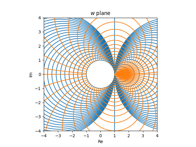
At the end of the post I noted that evenly distributed grid lines in the z plane result in very unevenly spaced circles on the Smith chart in the w plane. We can fill in the Smith chart how we please by working backward, starting from a desired spacing of circles in the chart and tracing them back to the z plane.

The inverse of the function f is

g(w) = (1 + w)/(1 − w).

Complete circles

The Smith chart contains two kinds of circles: circles that fit entirely inside the chart, which are the images of vertical lines in the z plane, and circles that extend outside the chart, which are the images of horizontal lines. In the image below, the former are blue and the latter are orange.

We can space out the complete (blue) circles how we wish and use the inverse transformation g(w) to determine the corresponding spacing of the vertical lines in the z plane. If we take a point w₀ along the horizontal diameter of the Smith chart, w₀ is a real number, and so is its inverse z₀ = g(w₀).

So if we’d like the intersections of the complete circles with the diameter to be uniformly spaced, we pick uniformly spaced points w_i and use as our vertical lines in the z plane the lines with real part g(w_i).

Here’s the image we’d get if we wanted circles passing through the diameter of the Smith chart at increments of 0.1.

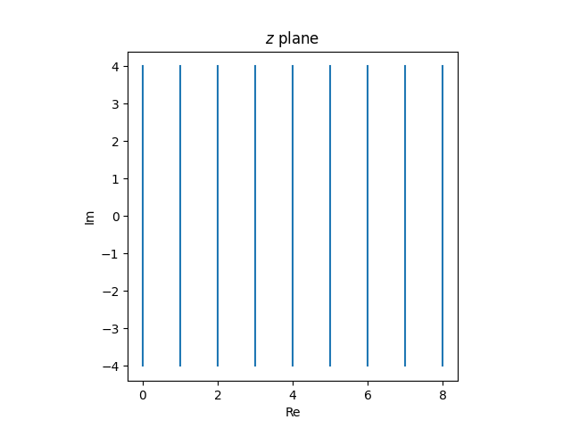
And here’s the corresponding set of vertical lines in the z plane that would produce these circles.

Incomplete circles

Now onto the incomplete circles, the orange circles in the graph above that are perpendicular to the blue circles.

As we showed in the previous post, the outer rim of the Smith chart is the image of the imaginary axis in the z plane under the function f(z). So if we pick a point w_i on the rim that we’d like a circle to pass through, we use the horizontal line with imaginary part equal to g(w_i).

So if we wanted orange circles to cross the boundary of the Smith chart every 10°, we pick w‘s from the interval [−π, π] spaced π/18 apart.

We can create these lines on the Smith chart below

from these lines in the z plane.

Putting it all together

The image of this grid in the z plane

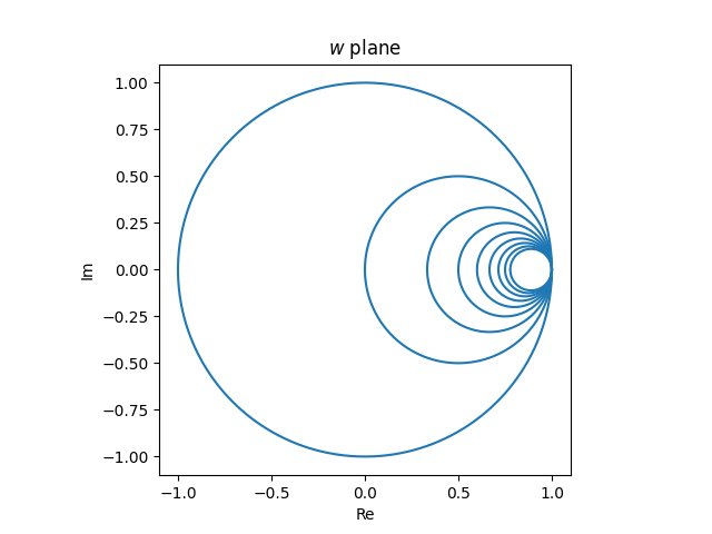
is the following in the w plane.

Compromise

The Smith charts printed in textbooks use some compromise between even spacing in the w plane and even spacing in the z plane.

Smith chart

How to make a Smith chart

Posted on 23 October 2025 by John

The Smith chart from electrical engineering is the image of a Cartesian grid under the function

f(z) = (z − 1)/(z + 1).

More specifically, it’s the image of a grid in the right half-plane.

Smith chart

This post will derive the basic mathematical properties of this graph but will not go into the applications. Said another way, I’ll explain how to make a Smith chart, not how to use one.

We will use z to denote points in the right half-plane and w to denote the image of these points under f. We will speak of lines in the z plane and the circles they correspond to in the w plane.

Möbius transformations

Our function f is a special case of a Möbius transformation. There is a theorem that says Möbius transformation map generalized circles to generalized circles. Here a generalized circle means a circle or a line; you can think of a line as a circle with infinite radius. We’re going to get a lot of mileage out of that theorem.

Image of the imaginary axis

The function f maps the imaginary axis in the z plane to the unit circle in the w plane. We can prove this using the theorem above. The imaginary axis is a line, so it’s image is either a line or a circle. We can take three points on the imaginary axis in the z plane and see where they go.

When we pick z equal to 0, i, and −i from the imaginary axis we get w values of −1, i, and −i. These three w values do not line on a line, so the image of the imaginary axis must be a circle. Furthermore, three points uniquely determine a circle, so the image of the imaginary axis is the circle containing −1, i, and −i, i.e. the unit circle.

Image of the right half-plane

The imaginary axis is the boundary of the right half-plane. Since it is mapped to the unit circle, the right half-plane is either mapped to the interior of the unit circle or the exterior of the unit circle. The point z = 1 goes to w = 0, and so the right half-plane is mapped inside the unit circle.

Images of vertical lines

Let’s think about what happens to vertical lines in the z plane, lines with constant positive real part. The images of these lines in the w plane must be either lines or circles. And since the right-half plane gets mapped inside the unit circle, these lines must get mapped to circles.

We can say a little more. All lines contain the point ∞, and f(∞) = 1, so the image of every vertical line in the z plane is a circle in the w plane, inside the unit circle and tangent to the unit circle at w = 1. (Tossing around ∞ is a bit informal, but it’s easy to make rigorous.)

The vertical lines in the z plane

map to tangent circles in the w plane.

Images of horizontal lines

Next, let’s think about horizontal lines in the z plane, lines with constant imaginary part. The image of these lines is either a line or a circle. Which is it? The image of a line is a line if it contains ∞, otherwise it’s a circle. Now f(z) = ∞ if and only if z = −1, and so the image of the real axis is a line, but the image of every other horizontal line is a circle.

Since f(∞) = 1, the image of every horizontal line passes through 1, just as the images of all the vertical lines passes through 1.

Since horizontal lines extend past the right half-plane, the image circles extend past the unit circle. The part of the line with positive real part gets mapped inside the unit circle, and the part of the line with negative real part gets mapped outside the unit circle. In particular, the image of the positive real axis is the interval [−1, 1].

Möbius transformations are conformal maps, and so they preserve angles of intersection. Since horizontal lines are perpendicular to vertical lines, the circles that are the images of the horizontal lines meet the circles that are the images of vertical lines at right angles.

The horizontal rays in the z plane

become partial circles in the w plane.

If we were to look at horizontal lines rather than rays, i.e. if we extended the lines into the left half-plane, the images in the w plane would be full circles.

Now let’s put our images together. The grid

in the z plane becomes the following in the w plane.

Spacing

An evenly spaced grid in the z plane becomes a very unevenly spaced graph in the w plane. Things are crowded on the right hand side and sparse on the left. A useable Smith chart needs to be roughly evenly filled in, which means it has to be the image of an unevenly filled in grid in the z plane. For example, you’d need more vertical lines in the z plane with small real values than with large real values.

I address the issue of spacing in the next post.

Generating random points in Colorado

Posted on 22 October 2025 by John

The previous post looked at how to generate random points on a sphere, generating spherical coordinates directly. I wanted to include a demonstration that this generates points with the same distribution as the more customary way of generating points on a sphere, and then decided the demonstration should be its own post.

I’ll generate random points in Colorado using both methods and show that both put the same proportion of points in the state, within a margin that we’d expect from random points.

I thought about using Wyoming, because I’ve been there recently, or Kansas, because I’m going there soon. Although Wyoming and Kansas are essentially rectangles, there are minor complications to the coordinates of the corners. But Colorado is very simple: it’s bounded by latitudes 37°N and 41°N and by longitudes 102.05°W and 109.05°W.

Here are the two ways of generating points on a sphere.

from numpy import *

# Random point on unit sphere in spherical coordinates
def random_spherical():
    rho = 1
    theta = 2*pi*random.random()
    phi = arccos(1 - 2*random.random())
    return (rho, theta, phi)

# Random point on unit sphere in Cartesian coordinates
def random_cartesian():
    v = random.normal(size=3)
    return v / linalg.norm(v)

We’ll need to convert Cartesian coordinates to spherical coordinates.

def cartesian_to_spherical(v):
    rho = linalg.norm(v)
    theta = arctan2(v[1], v[0])
    phi = arccos(v[2] / rho)
    return (rho, theta, phi)

And we’ll need to convert spherical coordinates to latitude and longitude in degrees. Note that latitude is π/2 minus the polar angle.

def spherical_to_lat_long(rho, theta, phi):
    lat = rad2deg(pi/2 - phi)
    long = rad2deg(theta)
    return (lat, long)

And finally, we need a way to test whether a (lat, long) pair is in Colorado.

def in_colorado(lat, long):
    return (37 <= lat < 41) and (102.05 <= long <= 109.05)

Now we’ll generate a million random points each way and count how many land in Colorado.

random.seed(20251022)
N = 1_000_000

count = 0
for _ in range(N):
    rho, theta, phi = random_spherical()
    lat, long = spherical_to_lat_long(rho, theta, phi)
    if in_colorado(lat, long):
        count += 1
print(count / N)

count = 0
for _ in range(N):
    v = random_cartesian()
    rho, theta, phi = cartesian_to_spherical(v)
    lat, long = spherical_to_lat_long(rho, theta, phi)
    if in_colorado(lat, long):
        count += 1
print(count / N)

This prints 0.000534 and 0.000536.

Efficiency

Note that this isn’t a very efficient way to generate points in Colorado since only about 5 out of every 10,000 points land in the state. If you wanted to generate points only in Colorado, you could randomly generate latitudes between 37° and 41°N and randomly generate longitudes 102.05° and 109.05°. This might be good enough in practice, depending on the application, but it’s not quite right because Colorado is not a Euclidean rectangle but a spherical rectangle.

A more accurate approach would be to randomly generate longitudes 102.05° and 109.05° as above, but generate latitudes as the arccos of points uniformly generated between cos(37°) and cos(41°).

Random spherical coordinates

Posted on 22 October 2025 by John

The topic of generating random points on a unit sphere has come up several times here. The standard method using normal random samples generates points (x, y, z) in Cartesian coordinates.

If you wanted points in spherical coordinates, you could first generate points in Cartesian coordinates, then convert the points to spherical coordinates. But it would seem more natural, and possibly more efficient, to directly generate spherical coordinates (ρ, θ, ϕ). That’s what we’ll do in this post.

Unfortunately there are several conventions for spherical coordinates, as described here, so we should start by saying we’re using the math convention that (ρ, θ, ϕ) means (radius, longitude, polar angle). The polar angle ϕ is 0 at the north pole and π at the south pole.

Generating the first two spherical coordinate components is trivial. On a unit sphere, ρ = 1, and θ we generate uniformly on [0, 2φ]. The polar angle ϕ requires more thought. If we simply generated φ uniformly from [0, π] we’d put too many points near the poles and too few points near the equator.

As I wrote about a few days ago, the x, y, and z coordinates of points on a sphere are uniformly distributed. In particular, the z coordinate is uniformly distributed, and so we need cos ϕ to be uniformly distributed, not ϕ itself. We can accomplish this by generating uniform points from [−1, 1] and taking the inverse cosine.

Here’s Python code summarizing the algorithm for generating random points on a sphere in spherical coordinates.

from numpy import random, pi, arccos

def random_pt() # in spherical coordinates
    rho = 1
    theta = 2*pi*random.random()
    phi = arccos(1 - 2*random.random())
    return (rho, theta, phi)

See the next post for a demonstration.

Distribution of correlation

Posted on 20 October 2025 by John

One of the more subtle ideas to convey in an introductory statistics class is that statistics have distributions.

Students implicitly think that when you calculate a statistic on a data set, say the mean, that then you have THE mean. But if your data are (modeled as) samples from a random variable, then anything you compute from those samples, such as the mean, is also a random variable. When you compute a useful statistic, it’s not as random as the data, i.e. it has smaller variance, but it’s still random.

A couple days ago I wrote about Fisher’s transform to make the distribution sample correlations closer to normal. This post will make that more concrete.

Preliminaries

We’ll need to bring in a few Python libraries. While we’re at it, let’s set the random number generator seed so the results will be reproducible.

import numpy as np
import matplotlib.pyplot as plt
from scipy.stats import skew

np.random.seed(20251020)

Correlated RNG

Next, we’ll need a way to generate correlated random samples, specifying the correlation ρ and the sample size N.

def gen_correlated_samples(rho, N):
    mean = [0, 0]
    cov = [
        [1, rho],
        [rho, 1]
    ]
    return np.random.multivariate_normal(mean, cov, size=N)

Calculating correlation

Once we generate correlated pairs, we need to calculate their correlation. To be more precise, their linear (Pearson) correlation. To do this we’ll find the empirical covariance matrix, the sample counterpart to the covariance matrix specified in the generator code above. The correlation coefficient is then the off-diagonal element of the covariance matrix.

def pearsonr(X):
    correlation_matrix = np.corrcoef(X[:,0], X[:,1])
    return correlation_matrix[0, 1]

Simulation

Now we’re ready to do our simulation.

M = 10000
rs = np.zeros(M)
for i in range(M):
    X = gen_correlated_samples(0.9, 100)
    rs[i] = pearsonr(X)

Notice that there are two levels of sampling. We’re generating random samples of size 100 and computing their correlation; that’s sampling our underlying data. And we’re repeating the process of computing the correlation 10,000 times; that’s sampling the correlation.

Untransformed distribution

Next we view the distribution of the correlation values.

plt.hist(rs, bins=int(np.sqrt(M)))
plt.show()
plt.close()

This gives the following plot.

It’s strongly skewed to the left, which we can quantify by calculating the skewness.

print(skew(rs))

This tells us the skewness is −0.616. A normal distribution has skewness 0. The negative sign tells us the direction of the skew.

Transformed distribution

Now let’s apply the Fisher transformation and see how it makes the distribution much closer to normal.

xformed = np.arctanh(rs)
plt.hist(xformed, bins=int(np.sqrt(M)))
plt.show()
plt.close()
print(skew(xformed))

This produces the plot below and prints a skewness value of −0.0415.

Small correlation example

We said before that when the correlation ρ is near zero, the Fisher transformation is less necessary. Here’s an example where ρ = 0.1. It’s not visibly different from a normal distribution, and the skewness is −0.1044.

Observation and conjecture

In our two examples, the skewness was approximately −ρ. Was that a coincidence, or does that hold more generally? We can test this with the following code.

def skewness(rho):
    rs = np.zeros(M)
    for i in range(M):
        X = gen_correlated_samples(rho, 100)
        rs[i] = pearsonr(X)
    return skew(rs)
    
rhos = np.linspace(-1, 1, 100)
ks = [skewness(rho) for rho in rhos]
plt.plot(rhos, ks)
plt.plot(rhos, -rhos, "--", color="gray")
plt.show()

Here’s the resulting plot.

It looks like the skewness is not exactly −ρ, but −cρ for some c < 1. Maybe c depends on the inner sample size, in our case 100. But it sure looks like skewness is at least approximately proportional to ρ. Maybe this is a well-known result, but I haven’t seen it before.

Author: John