Science versus medicine

Before I started working for a cancer center, I was not aware of the tension between science and medicine. Popular perception is that the two go together hand and glove, but that’s not always true.

Physicians are trained to use their subjective judgment and to be decisive. And for good reason: making a fairly good decision quickly is often better than making the best decision eventually. But scientists must be tentative, withhold judgment, and follow protocols.

Sometimes physician-scientists can reconcile their two roles, but sometimes they have to choose to wear one hat or the other at different times.

The physician-scientist tension is just one facet of the constant tension between treating each patient effectively and learning how to treat future patients more effectively. Sometimes the interests of current patients and future patients coincide completely, but not always.

This ethical tension is part of what makes biostatistics a separate field of statistics. In manufacturing, for example, you don’t need to balance the interests of current light bulbs and future light bulbs. If you need to destroy 1,000 light bulbs to find out how to make better bulbs in the future, no big deal. But different rules apply when experimenting on people. Clinical trials will often use statistical designs that sacrifice some statistical power in order to protect the people participating in the trial. Ethical constraints make biostatistics interesting.

Probability that a study result is true

Suppose a new study comes out saying a drug or a food or a habit lowers your risk of some disease. What is the probability that the study’s result is correct? Obviously this is a very important question, but one that is not raised often enough.

I’ve referred to a paper by John Ioannidis (*) several times before, but I haven’t gone over the model he uses to support his claim that most study results are false. This post will look at some equations he derives for estimating the probability that a claimed positive result is correct.

First of all, let R be the ratio of positive findings to negative findings being investigated in a particular area. Of course we never know exactly what R is, but let’s pretend that somehow we knew that out of 1000 hypotheses being investigated in some area, 200 are correct. Then R would be 200/800 = 0.25. The value of R varies quite a bit, being relatively large in some fields of study and quite small in others. Imagine researchers pulling hypotheses to investigate from a hat. The probability of selecting a hypothesis that really is true would be R/(R+1) and the probability selecting a false hypothesis is 1/(R+1).

Let α be the probability of incorrectly declaring a false hypothesis to be true. Studies are often designed with the goal that α would be 0.05. Let β be the probability that a study would incorrectly conclude that that a true hypothesis is false. In practice, β is far more variable than α. You might find study designs with β anywhere from 0.5 down to 0.01. The design choice β = 0.20 is common in some contexts.

There are two ways to publish a study claiming a new result: you could have selected a true hypothesis and correctly concluded that it was true, or you could have selected a false but incorrectly concluded it was true. The former has probability (1-β)R/(R+1) and the latter has probability α/(R+1). The total probability of concluding a hypothesis is true, correctly or incorrectly, is the sum of these probabilities, i.e. ((1-β)R + α)/(R+1). The probability that a study conclusion is true given that you concluded it was true, the positive predictive value or PPV, is the ratio of (1-β)R/(R+1) to ((1-β)R + α)/(R+1). In summary, under the assumptions above, the probability of a claimed result being true is (1-β)R/((1-β)R + α).

If (1 – β)R < α then the model say that a claim is more likely to be false than true. This can happen if R is small, i.e. there are not a large proportion of true results under investigation, and if β is large, i.e. if studies are small. If R is smaller than α, most studies will be false no matter how small you make β, i.e. no matter how large the study. This says that in a challenging area, where few of the ideas being investigated lead to progress, there will be a large proportion of false results published, even if the individual researchers are honest and careful.

Ioannidis develops two other models refining the model above. Suppose that because of bias, some proportion of results that would otherwise have been reported as negative are reported as positive. Call this proportion u. The derivation of the positive predictive value is similar to that in the previous model, but messier. The final result is R(1-β + uβ)/(R(1-β + uβ) + α + u – αu). If 1 – β > α, which is nearly always the case, then the probability of a reported result being correct decreases as bias increases.

The final model considers the impact of multiple investigators testing the same hypothesis. If more people try to prove the same thing, it’s more likely that someone will get lucky and “prove” it, whether or not the thing to be proven is true. Leaving aside bias, if n investigators are testing each hypothesis, the probability that a positive claim is true is given by R(1 – βn)/(R + 1 – (1 – α)nRβn). As n increases, the probability of a positive claim being true decreases.

The probability of a result being true is often much lower than is commonly believed. One reason is that hypothesis testing focuses on the probability of the data given a hypothesis rather than the probability of a hypothesis given the data. Calculating the probability of a hypothesis given data relies on prior probabilities, such as the factors R/(R+1) and 1/(R+1) above. These prior probabilities are elusive and controversial, but they are critical in evaluating how likely it is that claimed results are true.

Related: Adaptive clinical trial design


(*) John P. A. Ioannidis, Why most published research findings are false. CHANCE volume 18, number 4, 2005.

Sometimes it’s right under your nose

Neptune was discovered in 1846. But Galileo’s notebooks describe a “star” he saw on 28 December 1612 and 2 January 1613 that we now know was Neptune. Galileo even noticed that his star was in a slightly different location for his two observations, but he chalked the difference up to observational error.

The men who discovered Neptune were not the first to see it; they were the first to realize what they were looking at.

Drug looks promising, come back in 30 years

The most recent 60-Second Science podcast summarizes a paper in Science magazine reporting that the average interval between a drug being deemed “promising” and the first paper appearing showing clinical effectiveness is 24 years.

Note that the publication of a paper saying a drug is clinically effective is a far cry from regulatory approval. Many new drugs that look like an improvement after a phase II trial turn out to be no better than existing treatments, and those really are better take years to achieve regulatory approval.

* * *

Consulting in clinical trial design

Random inequalities VII: three or more variables

The previous posts in this series have looked at P(X > Y), the probability that a sample from a random variable X is greater than a sample from an independent random variable Y. In applications, X and Y have different distributions but come from the same distribution family.

Sometimes applications require computing P(X > max(Y, Z)). For example, an adaptively randomized trial of three treatments may be designed to assign a treatment with probability equal to the probability that that treatment has the best response. In a trial with a binary outcome, the variables X, Y, and Z may be beta random variables representing the probability of response. In a trial with a time-to-event outcome, the variables might be gamma random variables representing survival time.

Sometimes we’re interested in the opposite inequality, P(X < min(Y,Z)). This would be the case if we thought in terms of failures rather than responses, or wanted to minimize the time to a desirable event rather than maximizing the time to an undesirable event.

The maximum and minimum inequalities are related by the following equation:

P(X < min(Y,Z)) = P(X > max(Y, Z)) + 1 – P(X > Y) – P(X > Z).

These inequalities are used for safety monitoring rules as well as to determine randomization probabilities. In a trial seeking to maximize responses, a treatment arm X might be dropped if P(X > max(Y,Z)) becomes too small.

In principle one could design an adaptively randomized trial with n treatment arms for any n ≥ 2 based on P(X1 > max(X2, …, Xn)). In practice, the most common value of n by far is 2. Sometimes n is 3. I’m not familiar with an adaptively randomized trial with more than three arms. I’ve heard of an adaptively randomized trial that was designed with five arms, but I don’t believe the trial ran.

Computing P(X1 > max(X2, …, Xn)) by numerical integration becomes more difficult as n increases. For large n, simulation may be more efficient than integration. Computing P(X1 > max(X2, …, Xn)) for gamma random variables with n=3 was unacceptably slow in a previous version of our adaptive randomization software. The search for a faster algorithm lead to this paper: Numerical Evaluation of Gamma Inequalities.

Previous posts on random inequalities:

Random inequalities VI: gamma distributions

This post looks at computing P(X > Y) where X and Y are gamma random variables. These inequalities are central to the Thall-Wooten method of monitoring single-arm clinical trials with time-to-event outcomes. They also are central to adaptively randomized clinical trials with time-to-event outcomes.

When X and Y are gamma random variables P(X > Y) can be computed in terms of the incomplete beta function. Suppose X has shape αX and scale βX and Y has shape αY and scale βY. Then βXY/(βX Y+ βYX) has a beta(αY, αX) distribution. (This result is well-known in the special case of the scale parameters both equal to 1. I wrote up the more general result here but I don’t imagine I was the first to stumble on the generalization.) It follows that

P(X < Y) = P(B < βX/(βX+ βY))

where B is a beta(αY, αX) random variable.

For more details, see Numerical evaluation of gamma inequalities.

Previous posts on random inequalities:

Stopping trials of ineffective drugs earlier

Valen Johnson and I recently posted a working paper on a method for stopping trials of ineffective drugs earlier. For Bayesians, we argue that our method is more consistently Bayesian than other methods in common use. For frequentists, we show that our method has better frequentist operating characteristics than the most commonly used safety monitoring method.

The paper looks at binary and time-to-event trials. The results are most dramatic for the time-to-event analog of the Thall-Simon method, the Thall-Wooten method, as shown below.

This graph plots the probability of concluding that an experimental treatment is inferior when simulating from true mean survival times ranging from 2 to 12 months. The trial is designed to test a null hypothesis of 6 months mean survival against an alternative hypothesis of 8 months mean survival. When the true mean survival time is less than the alternative hypothesis of 8 months, the Bayes factor design is more likely to stop early. And when the true mean survival time is greater than the alternative hypothesis, the Bayes factor method is less likely to stop early.

The Bayes factor method also outperforms the Thall-Simon method for monitoring single-arm trials with binary outcomes. The Bayes factor method stops more often when it should and less often when it should not. However, the difference in operating characteristics is not as pronounced as in the time-to-event case.

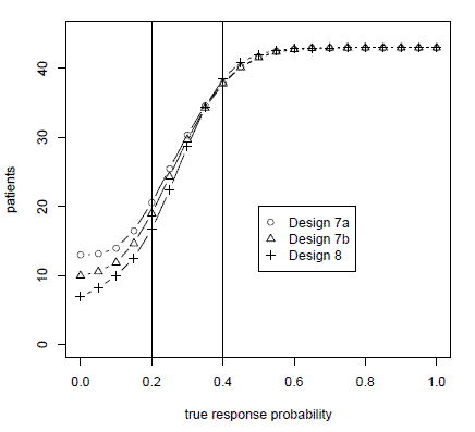
The paper also compares the Bayes factor method to the frequentist mainstay, the Simon two-stage design. Because the Bayes factor method uses continuous monitoring, the method is able to use fewer patients while maintaining the type I and type II error rates of the Simon design as illustrated in the graph below.

bayes factor vs simon two-stage designs

The graph above plots the number of patients used in a trial testing a null hypothesis of a 0.2 response rate against an alternative of a 0.4 response rate. Design 8 is the Bayes factor method advocated in the paper. Designs 7a and 7b are variations on the Simon two-stage design. The horizontal axis gives the true probabilities of response. We simulated true probabilities of response varying from 0 to 1 in increments of 0.05. The vertical axis gives the number of patients treated before the trial was stopped. When the true probability of response is less than the alternative hypothesis, the Bayes factor method treats fewer patients. When the true probability of response is better than the alternative hypothesis, the Bayes factor method treats slightly more patients.

Design 7a is the strict interpretation of the Simon method: one interim look at the data and another analysis at the end of the trial. Design 7b is the Simon method as implemented in practice, stopping when the criteria for continuing cannot be met at the next analysis. (For example, if the design says to stop if there are three or fewer responses out of the first 15 patients, then the method would stop after the 12th patient if there have been no responses.) In either case, the Bayes factor method uses fewer patients. The rejection probability curves, not shown here, show that the Bayes factor method matches (actually, slightly improves upon) the type I and type II error rates for the Simon two-stage design.

Related: Adaptive clinical trial design

Random inequalities V: beta distributions

I’ve put a lot of effort into writing software for evaluating random inequality probabilities with beta distributions because such inequalities come up quite often in application. For example, beta inequalities are at the heart of the Thall-Simon method for monitoring single-arm trials and adaptively randomized trials with binary endpoints.

It’s not easy to evaluate P(X > Y) accurately and efficiently when X and Y are independent random variables. I’ve seen several attempts that were either inaccurate or slow, including a few attempts on my part. Efficiency is important because this calculation is often in the inner loop of a simulation study. Part of the difficulty is that the calculation depends on four parameters and no single algorithm will work well for all parameter combinations.

Let g(a, b, c, d) equal P(X > Y) where X ~ beta(a, b) and Y ~ beta(c, d). Then the function g has several symmetries.

  • g(a, b, c, d) = 1 – g(c, d, a, b)
  • g(a, b, c, d) = g(d, c, b, a)
  • g(a, b, c, d) = g(d, b, c, a)

The first two relations were published by W. R. Thompson in 1933, but as far as I know the third relation first appeared in this technical report in 2003.

For special values of the parameters, the function g(a, b, c, d) can be computed in closed form. Some of these special cases are when

  • one of the four parameters is an integer
  • a + b + c + d = 1
  • a + b = c + d = 1.

The function g(a, b, c, d) also satisfies several recurrence relations that make it possible to bootstrap the latter two special cases into more results. Define the beta function B(a, b) as Γ(a, b)/(Γ(a) Γ(b)) and define h(a, b, c, d) as B(a+c, b+d)/( B(a, b) B(c, d) ). Then the following recurrence relations hold.

  • g(a+1, b, c, d) = g(a, b, c, d) + h(a, b, c, d)/a
  • g(a, b+1, c, d) = g(a, b, c, d) – h(a, b, c, d)/b
  • g(a, b, c+1, d) = g(a, b, c, d) – h(a, b, c, d)/c
  • g(a, b, c, d+1) = g(a, b, c, d) + h(a, b, c, d)/d

For more information about beta inequalities, see these papers:

Previous posts on random inequalities: