Conflicting ideas of simplicity

Sometimes it’s simpler to compute things exactly than to use an approximation. When you work on problems that cannot be computed exactly long enough, you start to assume everything falls in that category. I posted a tech report a few days ago about a problem in studying clinical trials that could be solved exactly even though it was commonly approximated by simulation.

This is another example of trying the simplest thing that might work. But it’s also an example of conflicting ideas of simplicity. It’s simpler, in a sense, to do what you’ve always done than to do something new.

It’s also an example of a conflict between a programmer’s idea of simplicity versus a user’s idea of simplicity. For this problem, the slower and less accurate code requires less work. It’s more straightforward and more likely to be correct. The exact solution takes less code but more thought, and I didn’t get it right the first time. But from a user’s perspective, having exact results is simpler in several ways: no need to specify a number of replications, no need to wait for results, no need to argue over what’s real and what’s simulation noise, etc. In this case I’m the programmer and the user so I feel the tug in both directions.

Subjecting fewer patients to ineffective treatments

Tomorrow morning I’m giving a talk on how to subject fewer patients to ineffective treatment in clinical trials. I should have used something like the title of this post as the title of my talk, but instead my talk is called “Clinical Trial Monitoring With Bayesian Hypothesis Testing.” Classic sales mistake: emphasizing features rather than benefits. But the talk is at a statistical conference, so maybe the feature-oriented title isn’t so bad.

Ethical concerns are the main consideration that makes biostatistics a separate branch of statistics. You can’t test experimental drugs on people the way you test experimental fertilizers on crops. In human trials, you want to stop the trial early if it looks like the experimental treatment is not as effective as a comparable established treatment, but you want to keep going if it looks like the new treatment might be better. You need to establish rules before the trial starts that quantify exactly what it means to look like a treatment is doing better or worse than another treatment. There are a lot of ways of doing this quantification, and some work better than others. Within its context (single-arm phase II trials with binary or time-to-event endpoints) the method I’m presenting stops ineffective trials sooner than the methods we compare it to while stopping no more often in situations where you’d want the trial to continue.

If you’re not familiar with statistics, this may sound strange. Why not always stop when a treatment is worse and never stop when it’s better? Because you never know with certainty that one treatment is better than another. The more patients you test, the more sure you can be of your decision, but some uncertainty always remains. So you face a trade-off between being more confident of your conclusion and experimenting on more patients. If you think a drug is bad, you don’t want to treat thousands more patients with it in order to be extra confident that it’s bad, so you stop. But you run the risk of shutting down a trial of a treatment that really is an improvement but by chance appeared to be worse at the time you made the decision to stop. Statistics is all about such trade-offs.

Related: Adaptive clinical trial design

Random inequalities I: introduction

Many Bayesian clinical trial methods have at their core a random inequality. Some examples from M. D. Anderson: adaptive randomization, binary safety monitoring, time-to-event safety monitoring. These method depends critically on evaluating P(X > Y) where X and Y are independent random variables. Roughly speaking, P(X > Y) is the probability that the treatment represented by X is better than the treatment represented by Y. In a trial with binary outcomes, X and Y may be the posterior probabilities of response on each treatment. In a trial with time-to-event outcomes, X and Y may be posterior probabilities of median survival time on two treatments.

People often have a little difficulty understanding what P(X > Y) means. What does it mean? If we take a sample from X and a random sample from Y, P(X >Y) is the probability that the former is larger than the latter. Most confusion around random inequalities comes from thinking of random variables as constants, not random quantities. Here are a couple examples.

First, suppose X and Y have normal distributions with standard deviation 1. If X has mean 4 and Y has mean 3, what is P(X > Y)? Some would say 1, because X is bigger than Y. But that’s not true. X has a larger mean than Y, but fairly often a sample from Y will be larger than a sample from XP(X > Y) = 0.76 in this case.

Next, suppose X and Y are identically distributed. Now what is P(X > Y)? I’ve heard people say zero because the two random variables are equal. But they’re not equal. Their distribution functions are equal but the two random variables are independent. P(X > Y) = 1/2 by symmetry.

I believe there’s a psychological tendency to underestimate large inequality probabilities. (I’ve had several discussions with people who would not believe a reported inequality probability until they computed it themselves. These discussions are important when the decision whether to continue a clinical trial hinges on the result.) For example, suppose X and Y represent the probability of success in a trial in which there were 17 successes out of 30 on X and 12 successes out of 30 on Y. Using a beta distribution model, the density functions of X and Y are given below.

beta inequality graph

The density function for X is essentially the same as Y but shifted to the right. Clearly P(X > Y) is greater than 1/2. But how much greater than a half? You might think not too much since there’s a lot of mass in the overlap of the two densities. But P(X > Y) is a little more than 0.9.

The image above and the numerical results mentioned in this post were produced by the Inequality Calculator software.

Part II will discuss analytically evaluating random inequalities. Part III will discuss numerically evaluating random inequalities.

Three ways of tuning an adaptively randomized trial

Yesterday I gave a presentation on designing clinical trials using adaptive randomization software developed at M. D. Anderson Cancer Center. The heart of the presentation is summarized in the following diagram.
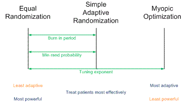
Diagram of three methods of tuning adaptively randomized trial designs

(A slightly larger and clearer version if the diagram is available here.)

Traditional randomized trials use equal randomization (ER). In a two-arm trial, each treatment is given with probability 1/2. Simple adaptive randomization (SAR) calculates the probability that a treatment is the better treatment given the data seen so far and randomizes to that treatment with that probability. For example, if it looks like there’s an 80% chance that Treatment B is better, patients will be randomized to Treatment B with probability 0.80. Myopic optimization (MO) gives each patient what appears to be the best treatment given the available data with no randomization.

Myopic optimization is ethically appealing, but has terrible statistical properties. Equal randomization has good statistical properties, but will put the same number of patients on each treatment, regardless of the evidence that one treatment is better. Simple adaptive randomization is a compromise position, retaining much of the power of equal randomization while also treating more patients on the better treatment on average.

The adaptive randomization software provides three ways of compromising between the operating characteristics ER and SAR.

  1. Begin the trial with a burn-in period of equal randomization followed by simple adaptive randomization.
  2. Use simple adaptive randomization, except if the randomization probability drops below a certain threshold, substitute that minimum value.
  3. Raise the simple adaptive randomization probability to a power between 0 and 1 to obtain a new randomization probability.

Each of these three approaches reduces to ER at one extreme and SAR at the other. In between the extremes, each produces a design with operating characteristics somewhere between those of ER and SAR.

In the first approach, if the burn-in period is the entire trial, you simply have an ER trial. If there is no burn-in period, you have an SAR trial. In between you could have a burn-in period equal to some percentage of the total trial between 0 and 100%. A burn-in period of 20% is typical.

In the second approach, you could specify the minimum randomization probability as 0.5, negating the adaptive randomization and yielding ER. At the other extreme, you could set the minimum randomization probability to 0, yielding SAR. In between you could specify some non-zero randomization probability such as 0.10.

In the third approach, a power of zero yields ER. A power of 1 yields SAR. Unlike the other two approaches, this approach could yield designs approaching MO by using powers larger than 1. This is the most general approach since it can produce a continuum of designs with characteristics ranging from ER to MO. For more on this approach, see Understanding the exponential tuning parameter in adaptively randomized trials.

So with three methods to choose from, which one do you use? I did some simulations to address this question. I expected that all three methods would perform about the same. However, this is not what I found. To read more, see Comparing methods of tuning adaptive randomized trials.

Update: The ideas in this post and the technical report mentioned above have been further developed in this paper.

Related: Adaptive clinical trial design

Cohort assignments in clinical trials

Cohorts are very simple in theory but messy in practice. In a clinical trial, a cohort is a group of patients who receive the same treatment. For example, in dose-finding trials, it is very common to treat patients in groups of three. I’ll stick with cohorts of three just to be concrete, though nothing here depends particularly on this choice of cohort size.

If we number patients in the order in which they arrive, patients 1, 2, and 3 would be the first cohort. Patients 4, 5, and 6 would be the second cohort, etc. If it were always that simple, we could determine which cohort a patient belongs to based on their accrual number alone. To calculate a patient’s cohort number, subtract 1 from their accrual number, divide by 3, throw away any remainder, and add 1. In math symbols, the cohort number for patient #n would be 1 + ⌊(n-1)/3⌋. (See the next post.)

Here’s an example of why that won’t work. Suppose you treat patients 1, 2, and 3, then discover that patient #2 was not eligible for the trial after all. (This happens regularly.) Now a 4th patient enters the trial. What cohort are they in? If patient #4 arrived after you discovered that patient #2 was ineligible, you could put patient #4 in the first cohort, essentially taking patient #2’s place. But if patient #4 arrived before you discovered that patient #2 was ineligible, then patient #4 would receive the treatment assigned to the second cohort; the first cohort would have a hole in it and only contain two patients. You could treat patient #5 with the treatment of the first cohort to try to patch the hole, but that’s more confusing. It gets even worse if you’re on to the third or fourth cohort before discovering a gap in the first cohort.

In addition to patients being removed from a trial due to ineligibility, patients can remove themselves from a trial at any time.

There are numerous other ways the naïve view of cohorts can fail. A doctor may decide to give the same treatment to only two consecutive patients, or to four consecutive patients, letting medical judgment override the dose assignment algorithm for a particular patient. A mistake could cause a patient to receive the dose intended for another cohort. Researchers may be unable to access the software needed to make the dose assignment for a new cohort and so they give a new patient the dose from the previous cohort.

Cohort assignments can become so tangled that it is simply not possible to look at an ordered list of patients and their treatments after the fact and determine how the patients were grouped into cohorts. Cohort assignment is to some extent a mental construct, an expression of how the researcher thought about the patients, rather than an objective grouping.

Related: Adaptive clinical trial design
Small effective sample size does not mean uninformative

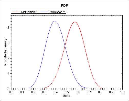
Today I talked to a doctor about the design of a randomized clinical trial that would use a Bayesian monitoring rule. The probability of response on each arm would be modeled as a binomial with a beta prior. Simple conjugate model. The historical response rate in this disease is only 5%, and so the doctor had chosen a beta(0.1, 1.9) prior so that the prior mean matched the historical response rate.

For beta distributions, the sum of the two parameters is called the effective sample size. There is a simple and natural explanation for why a beta(a, b) distribution is said to contain as much information as a+b data observations. By this criterion, the beta(0.1, 1.9) distribution is not very informative: it only has as much influence as two observations. However, viewed in another light, a beta(0.1, 1.9) distribution is highly informative.

This trial was designed to stop when the posterior probability is more than  0.999 that one treatment is more effective than the other. That’s an unusually high standard of evidence for stopping a trial — a cutoff of 0.99 or smaller would be much more common — and yet a trial could stop after only six patients. If X is the probability of response on one arm and Y is the probability of response on the other, after three failures on the first treatment and three successes on the other, Pr(Y > X) > 0.999.

The explanation for how the trial could stop so early is that the prior distribution is, in an odd sense, highly informative. The trial starts with a strong assumption that each treatment is ineffective. This assumption is somewhat justified by of experience, and yet a beta(0.1, 1.9) distribution doesn’t fully capture the investigator’s prior belief.

(Once at least one response has been observed, the beta(0.1, 1.9) prior becomes essentially uninformative. But until then, in this context, the prior is informative.)

A problem with a beta prior is that there is no way to specify the mean at 0.05 without also placing a large proportion of the probability mass below 0.05. The beta prior places too little probability on better outcomes that might reasonably happen. I imagine a more diffuse prior with mode 0.05 rather than mean 0.05 would better describe the prior beliefs regarding the treatments.

The beta prior is convenient because Bayes’ theorem takes a very simple form in this case: starting from a beta(a, b) prior and observing s successes and f failures, the posterior distribution is beta(a+s, b+f).  But a prior less convenient algebraically could be more robust and better adept at representing prior information.

A more basic observation is that “informative” and “uninformative” depend on context. This is part of what motivated Jeffreys to look for prior distributions that were equally (un)informative under a set of transformations. But Jeffreys’ approach isn’t the final answer. As far as I know, there’s no universally acceptable resolution to this dilemma.

Related: Adaptive clinical trial design

Galen and clinical trials

Here’s a quote from the Greek physician Galen (c. 130-210 A.D.)

All who drink of this remedy recover in a short time, except those whom it does not help, who all die. Therefore, it is obvious that it fails only in incurable cases.

Imagine a dialog between Galen and a modern statistician.

Stat: You say your new treatment is better than the previous one?

Galen: Yes.

Stat: But more people died on the new treatment.

Galen: Those patients don’t count because they were incurable. They would have died anyway.

The problem with Galen’s line of reasoning is that it is not falsifiable: no experiment could disprove it. He could call any treatment superior by claiming that evidence against it doesn’t count. Still, Galen might have been right.

Now suppose our statistician has a long talk with Galen and tells him about modern statistical technique.

Galen: Can’t you look back at my notes and see whether there was something different about the patients who didn’t respond to the new treatment? There’s got to be some explanation. Maybe my new treatment isn’t better for everyone, but there must be a group for whom it’s better.

Stat: Well, that’s tricky business. Advocates call that “subset analysis.” Critics call it “data dredging.” The problem is that the more clever you are with generating after-the-fact explanations, the more likely you’ll come up with one that seems true but isn’t.

Galen: I’ll have to think about that one. What do you propose we do?

Stat: We’ll have to do a randomized experiment. When each patient arrives, we’ll flip a coin to decide whether to give them the old or the new treatment. That way we expect about the same number of incurable patients to receive each treatment.

Galen: But the new treatment is better. Why should I give half my patients the worse treatment?

Stat: We don’t really know that the new treatment is better. Maybe it’s not. A randomized experiment will give us more confidence one way or another.

Galen: But couldn’t we be unlucky and assign more incurable patients to the better treatment?

Stat: Yes, that’s possible. But it’s not likely we will assign too many more incurable patients to either treatment. That’s just a chance we’ll have to take.

The issues in these imaginary dialogs come up all the time. There are people who believe their treatment is superior despite evidence to the contrary. But sometimes they’re right. New treatments are often tested on patients with poor prognosis, so the complaints of receiving more incurable patients are justified. And yet until there’s some evidence that a new treatment may be at least as good as standard, it’s unethical to give that treatment to patients with better prognosis. Sometimes post-hoc analysis finds a smoking gun, and sometimes it’s data dredging. Sometimes randomized trials fail to balance on important patient characteristics. There are no simple answers. Context is critical, and dilemmas remain despite our best efforts. That’s what makes biostatistics interesting.

Related: Adaptive clinical trial design


Randomized trials of parachute use

It is widely assumed that parachute use improves your chances of surviving a leap from an airplane. However, a meta analysis suggests this practice is not adequately supported by controlled experiments. See the article Parachute use to prevent death and major trauma related to gravitational challenge: systematic review of randomized controlled trials by Gordon C S Smith and Jill P Pell. The authors summarize their conclusions in the abstract.

As with many interventions intended to prevent ill health, the effectiveness of parachutes has not been subjected to rigorous evaluation by using randomised controlled trials. Advocates of evidence based medicine have criticised the adoption of interventions evaluated by using only observational data. We think that everyone might benefit if the most radical protagonists of evidence based medicine organised and participated in a double blind, randomised, placebo controlled, crossover trial of the parachute.

Dose-finding: why start at the lowest dose?

You’ve got a new drug and it’s time to test it on patients. How much of the drug do you give? That’s the question dose-finding trials attempt to answer.

The typical dose-finding procedure starts by selecting a small number of dose levels, say four or five. The trial begins by giving the lowest dose to the first few patients, and there is some procedure for deciding when to try higher doses. Convention says it is unethical to start at any dose other than lowest dose. I will give several reasons to question convention.

Suppose you want to run a clinical trial to test the following four doses of Agent X: 10 mg, 20 mg, 30 mg, 50 mg. You want to start with 20 mg. Your trial goes for statistical review and the reviewer says your trial is unethical because you are not starting at the lowest dose. You revise your protocol saying you only want to test three doses: 20 mg, 30 mg, and 50 mg. Now suddenly it is perfectly ethical to start with a dose of 20 mg because it is the lowest dose.

The more difficult but more important question is whether a dose of 20 mg of Agent X is medically reasonable. The first patient in the trial does not care whether higher or lower doses will be tested later. He only cares about the one dose he’s about to receive. So rather than asking “Why are you starting at dose 2?” reviewers should ask “How did you come up with this list of doses to test?”

A variation of the start-at-the-lowest-dose rule is the rule to always start at “dose 1”. Suppose you revise the original protocol to say dose 1 is 20 mg, dose 2 is 30 mg, and dose 3 is 50 mg. The protocol also includes a “dose -1” of 10 mg. You explain that you do not intend to give dose -1, but have included it as a fallback in case the lowest dose (i.e. 20 mg) turns out to be too toxic. Now because you call 20 mg “dose 1” it is ethical to begin with that dose. You could even begin with 30 mg if you were to label the two smaller doses “dose -2” and “dose -1.” With this reasoning, it is ethical to start at any dose, as long as you call it “dose 1.” This approach is justified only if the label “dose 1” carries the implicit endorsement of an expert that it is a medically reasonable starting dose.

Part of the justification for starting at the lowest dose is that the earliest dose-finding methods would only search in one direction. This explains why some people still speak of “dose escalation” rather than “dose-finding.” More modern dose-finding methods can explore up and down a dose range.

The primary reason for starting at the lowest dose is fear of toxicity. But when treating life-threatening diseases, one could as easily justify starting at the highest dose for fear of under treatment. (Some trials do just that.) Depending on the context, it could be reasonable to start at the lowest, highest, or any dose in between.

The idea of first selecting a range of doses and then deciding where to start exploring seems backward. It makes more sense to first pick the starting dose, then decide what other doses to consider.

Related: Adaptive clinical trial design