Confidential OCR

A client emailed me a screenshot of a table rather than pasting the table as text into an email.

I thought about using an LLM to convert it to text, but the table is confidential client information and so I shouldn’t upload it anywhere.

I searched for a commandline utility to do OCR and found tesseract. I installed it with

    sudo apt install tesseract-ocr libtesseract-dev tesseract-ocr-eng

and ran it with the default settings

    tesseract screenshot.png textfile

It worked remarkably well. I had to change a C to a U, but otherwise I didn’t have to add or change any text, but I did have to delete a few extraneous parentheses generated by the software.

I work locally in part out of habit; it was the only way to work when I started using a computer. It has numerous advantages, such as being able to keep working when a hurricane knocks out my internet connection, but above all it is private.

I pay more attention to privacy than is convenient because I work in data privacy. And aside from my privacy, I have to protect our clients’ privacy.

Update: According to the comments, ChatGPT uses tesseract. Assuming that’s true, using tesseract directly is better than ChatGPT because it does exactly what you want. No ambiguity as far as what expected. No potential for tinkering with your results before you see them.

Related posts

Resolving a mysterious problem with find

Suppose you want to write a shell script searches the current directory for files that have a keyword in the name of the file or in its contents. Here’s a first attempt.

find . -name '*.py' -type f -print0 | grep -i "$1"
find . -name '*.py' -type f -print0 | xargs -0 grep -il "$1"

This works well for searching file contents but behaves unexpectedly when searching for file names.

If I have a file named frodo.py in the directory, the script will return

grep: (standard input): binary file matches

Binary file matches?! I wasn’t searching binary files. I was searching files with names consisting entirely of ASCII characters. Where is a binary file coming from?

If we cut off the pipe at the end of the first line of the script and run

find . -name '*.py' -type f -print0

we get something like

.elwing.py/.frodo.py/gandalf.py

with no apparent non-ASCII characters. But if we pipe the output through xxd to see a hex dump, we see that there are invisible null characters after each file name.

One way to fix our script would be to add a -a option to the call to grep, telling to treat the input as ASCII. But this will return the same output as above. The output of find is treated as one long (ASCII) string, which matches the regular expression.

Another possibility would be to add a -o flag to direct grep to return just the match. But this is less than ideal as well. If you were looking for file names containing a Q, for example, you’d get Q as your output, which doesn’t tell you the full file name.

There may be better solutions [1], but my solution was to insert a call to strings in the pipeline:

find . -name '*.py' -type f -print0 | strings | grep -i "$1"

This will extract the ASCII strings out of the input it receives, which has the effect of splitting the string of file names into individual names.

By default the strings command defines an ASCII string to be a string of 4 or more consecutive ASCII characters. A file with anything before the .py extension will necessarily have at least four characters, but the analogous script to search C source files would overlook a file named x.c. You could fix this by using strings -n 3 to find sequences of three or more ASCII characters.

If you don’t have the strings command installed, you could use sed to replace the null characters with newlines.

find . -name '*.py' -type f -print0 | sed 's/\x0/\n/g' | grep -i "$1"

Note that the null character is denoted \x0 rather than simply \0.

Related posts

[1] See the comments for better solutions. I really appreciate your feedback. I’ve learned a lot over the years from reader comments.

Trigonometric interpolation

Suppose you want to interpolate a set of data points with a combination of sines and cosines.

One way to approach this problem would be to set up a system of equations for the coefficients of the sines and cosines. If you have N data points, you will get a system of N equations in N unknowns. The system will have a unique solution, though this is not obvious a priori.

Another approach would be to use the discrete Fourier transform (DFT). This is the approach that would commonly be used in practice. It’s even further from obvious a priori that this would work, but it does. (The DFT is so often computed using the FFT algorithm that the transform is often referred to by the algorithm name. If you’d like, mentally substitute FFT for DFT in the rest of the post.)

There are multiple ways to motivate the DFT, and the way suggested by the name is to derive the DFT as a discrete approximation to the (continuous) Fourier transform. Why should a discrete approximation to an integral transform also solve an interpolation problem? This doesn’t sound inevitable, or even plausible, but it is the case.

Another way to motivate the DFT is as the least-squares solution to fitting a sum of sines and cosines to a set of points. Since this is phrased as an optimization problem rather than an interpolation problem, it is clear that it will have a solution. However, it is not clear that the error in the optimal fit will in fact be zero. Furthermore, the equation for the coefficients in the solution is the same as the equation for the DFT. You can find a derivation in [1].

Example

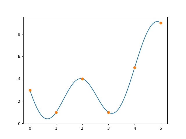
Let’s take the vector [3, 1, 4, 1, 5, 9] and find trig functions that pass through these points. We can use the FFT as implemented in Python’s SciPy library to find a set of complex exponentials that pass through the points.

    from scipy.fft import fft
    from numpy import exp, array, pi, round

    x = array([3, 1, 4, 1, 5, 9])
    y = fft(x)

    N = len(x)
    z = [sum([exp(2j*pi*k*n/N)*y[k] for k in range(N)])/N for n in range(N)]

Aside from rounding errors on the order of 10−15 the vector z equals the vector x.

Turning the expression for z above into a mathematical expression, we have

f(z) = y0 + y1 exp(nπi/3) + y2 exp(2nπi/3) + y3 exp(nπi) + y4 exp(4nπi/3) + y5 exp(5nπi/3)

where the y‘s come from the FFT above.

To find sines and cosines we need to use Euler’s formula

exp(iθ) = cos(θ) + i sin(θ)

Because started with real data x, there will be symmetries in the FFT components x that simplify the reduction of the complex function f to a real-valued function g using sines and cosines; some of the components will be conjugate and so the complex parts cancel out.

6 g(x) = y0 + (y1 + y5) cos(πx/3) + (y2 + y4) cos(2πx/3) + y3 cos(πx)
+ i (y1y5) sin(πx/3) + (y2y4) cos(2πx/3)

and so

g(x) = 3.833 + 0.8333 cos(πx/3) − 1.833 cos(2πx/3) + 0.1666 cos(πx)
− 2.5981 sin(πx/3) − 2.0207 cos(2πx/3)

Here’s a plot that verifies that g(x) passes through the specified points.

Related posts

[1] William L. Briggs and Van Emden Henson. The DFT: An Owner’s Manual for the Discrete Fourier Transform. SIAM 1995.

The impossible puzzle

It’s fascinating that there’s such a thing as the World Jigsaw Puzzle Championship. The winning team of the two-person thousand-piece puzzle round can assemble a Ravensburger puzzle in less than an hour—that’s about 3 -1/2 seconds per piece.

It makes you wonder, how could you measure the hardness of a jigsaw puzzle? And what would a “hardest puzzle” look like?

You can find some puzzles that are claimed to be “hardest.” A first step to creating a hard puzzle is removing the front image entirely, eliminating visual cues. Some puzzles do this. This can be partly simulated with a normal puzzle by putting it together with the image side face down.

But you can do more: make every piece a square exactly the same size, and the “tab“ and “blank“ on each of the four sides of each square exactly the same size, shape and alignment. One can see that this gives you 24 = 16 different unique kinds of puzzle piece, however, due to symmetries you actually have six different kinds of puzzle piece. Now, you are left with a bare minimum of shape cues to help you assemble the puzzle.

For the sake of the argument, one can ignore the “edge” pieces. One can see this from the fact that for a rectangular puzzle, as you scale up the size, the number of edge pieces proportional to the interior pieces of the puzzle becomes smaller and smaller. For example for a 36X28=1008 piece puzzle, there are (2*36+2*28-4)=124 edge pieces, about 12 percent of the whole. The ratio shrinks as you scale up puzzle size. And there is such a thing as a 42,000-piece jigsaw puzzle.

The solution complexity class for assembling such a puzzle is known to be NP-complete. This means that the best known algorithms require compute time that grows exponentially as the number of pieces is increased.

Of course there are simpler special cases. Consider a checkerboard configuration, in which “black square“ location pieces have four tabs and “red square” locations have four blanks, thus only two different kinds of piece. A competent puzzler could assemble this one piece per second, 17 minutes for a 1000-piece puzzle.

However, as far as we know, the number of “special cases” like this is vanishing small for large puzzles. An intuition for this can be taken from Kolmogorov complexity theory, using a counting argument to show that only very few long strings can be compressed to a short program.

Most cases are really hard, for example, constructed by making a totally random assignment for selecting the configuration of each piece-to-piece boundary. Solving this is really hard because you may have to backtrack: you may have the puzzle largely complete, but due to ambiguities, you may need to backtrack because of a wrong decision made early.

A very weak upper bound in the assembly time can be derived by considering the brute force case. For a 1000-piece puzzle, there are 1000! (factorial) possible ways to (attempt to) assemble the puzzle. Suppose one places every piece and then fully backtracks for each trial—this gives 1000 x 1000! puzzle piece placement steps. Using Stirling’s approximation, this is approximately 104468 placement steps.

A human, assuming generously a rate of one step per second, at 31 million seconds/year nonstop, would take on the order of 104460 years. Assuming 10 billion simultaneous puzzlers—order 104450 years.

Now assume the on-record world’s fastest computer, the ORNL Frontier system (though see here), roughly 10 exaflops (1019) mixed precision, and assuming one puzzle step per operation (overly optimistic). Assume further that every atom in the known universe (est. 1082) is a Frontier computer system. In this case—solving the puzzle takes order 104359 years. That’s a thousand billion billion … (repeat “billion” 484 times here) years.

As I mentioned, this is a very weak upper bound. One could solve the problem using a SAT solver with sophisticated CDCL backtracking. Or one could use special methods derived from statistical mechanics that handle random SAT instances. However, to the best of our knowledge, the runtime still grows exponentially as a function of puzzle size. The best worst-case computational complexity for SAT solvers currently known is order O(1.306995n) (see here, here, and here). So, simply by constructing puzzles in the way we’ve described with more and more pieces, you will soon reach a point of having a puzzle that is unfathomably difficult to solve.

It’s conceivable that a yet-undiscovered method could be found for which the solution cost would in fact grow polynomially instead of exponentially. But people have been trying to answer this question one way or the other for over 50 years and it’s still unsolved, with an open million dollar prize for proof or counterexample. So we just don’t know.

What about quantum computing? It can solve some exponential complexity problems like factoring in polynomial time. But how about the SAT problem? It is simply not known (see here, here) whether a polynomial-time quantum algorithm exists for arbitrary NP-complete problems. None are known, and it might not be possible at all (though research continues).

So we’re faced with the curious possibility: a jigsaw puzzle could be constructed for which, you’re holding the box of pieces in your hand, you spill it on the floor, and there is no single or joint intelligence or computational mechanism, existing or even possible, in the entire universe that could ever reassemble it.

Floating point: Everything old is new again

In the early days of computing hardware (and actually before) mathematicians put a lot of effort into understanding and mitigating the limitations of floating point arithmetic. They would analyze mundane tasks such as adding a list of numbers and think carefully about the best way to carry out such tasks as accurately as possible.

Now that most arithmetic is carried out in double precision, you can often get away with not thinking about such things. Except when you can’t. The vagaries of floating point computation still matter occasionally, even with double precision, though not as often as they did with single precision.

Although most computing has moved from single precision to double precision, there is increasing interest in going the opposite direction, from single precision to half precision. The main driver is neural networks. You don’t need a lot of precision in weights, and you’ve got a lot of numbers to store. So instead of taking 64 bits to store a double precision number, or 32 bits to store a single precision number. you might want to use a 16 bit or even 8 bit floating point number. That way you can fit more weights in memory at once.

However, when you move to lower precision numbers, you now have to think again about the things numerical analysts thought about a couple generations ago, such as different ways of rounding. You might think that floating point rounding could be modeled by random variables. If so, you’re in good company, because John von Neumann suggested this in 1947. But a few years later people began to realize that floating point rounding errors are not random. Or to be more precise, they began to realize that modeling rounding errors as random was inadequate; of course they knew that rounding errors weren’t literally random.

But what it rounding errors were random? This would lead to more error cancellation than we see in practice with floating point arithmetic. With stochastic rounding, the rounded values become unbiased estimators of the values they would like to represent but cannot represent exactly. Now the central limit theorem and all that come to your aid. More on applications of stochastic rounding here.

(To be pedantic a moment, stochastic rounding isn’t truly random, but uses pseudorandom numbers to implement a procedure which is well modeled by randomness. Random is as random does.)

Related posts

New Mersenne prime found

Mersenne numbers have the form 2p − 1. A Mersenne prime is a Mersenne number that is also a prime.

A new Mersenne prime discovery was announced today: 2p − 1 is prime for p = 136279841. The size of the new Mersenne prime is consistent with what was predicted.

For many years now, the largest known prime has been a Mersenne prime. That is because there is an special algorithm for testing whether a Mersenne number is prime, the Lucas-Lehmer test. Because of this algorithm, Mersenne numbers can be tested for primality far more efficiently than can arbitrary numbers of comparable size.

There are now 52 known Mersenne primes, but the number just announced may not be the 52nd Mersenne prime. It has been confirmed that the 2136279841 − 1 is prime, but it has not been confirmed that there are no Mersenne primes between the 51st Mersenne prime and the number just announced. There could be gaps.

If you were to write the latest Mersenne prime in hexadecimal, it would be a 1 followed by 34,069,960 F’s.

Related posts

RNG, PRNG, CSPRNG

Most random number generators are pseudorandom number generators (PRNGs). The distinction may be pedantic or crucial, depending on context. In the context of cryptography, it’s critical.

For this post, RNG will mean a physical, true random number generator.

A PRNG may be suitable for many uses—Monte Carlo simulation, numerical integration, game development, etc.—but not be suitable for cryptography. A PNRG which is suitable for cryptography is called a CSPRNG (cryptographically secure pseudorandom number generator).

A PRNG may have excellent statistical properties, and pass standard test suites for random number generators, and yet be insecure. The output of an insecure generator may have no statistical regularities, and yet have regularities that a sneaky cryptanalyst can exploit. For example, the popular Mersenne Twister is fine for simulations but its output can be predicted after a relatively short run. The prediction depends on a clever set of calculations that would be unnatural from a statistical perspective, which is why its statistical performance is better than its cryptographic performance.

CSPRNGs tend to be much slower than PRNGs, so you pay for security. And for a non-cryptographic application this cost isn’t worth it.

In general, statistical tests give necessary but not sufficient conditions for a PRNG to be a CSPRNG. If a PRNG fails statistical tests, it has some sort of regularity that potentially could be exploited by cryptanalysis. I had to tell a client once that although his PRNG passed the standard statistical tests, I was pretty sure I could break the cryptographic system he wanted to use it in. This news was not well received.

Lava lamp photo

I suspect that a physical RNG with good statistical properties will have good cryptographic properties as well, contrary to the usual case. Cloudflare famously uses lava lamps to generate random bits for TLS keys. Cryptanalysts have exploited minor flaws in PRNGs, and so the lava lamps give Cloudflare one less thing to worry about. (I’m sure they still have plenty else to worry about.)

A physical RNG might fail statistical tests. For example, maybe the physical process is truly random but biased. Or maybe the process of turning physical phenomena into numbers introduces some bias. But it’s hard to imagine that an RNG could have a clean bill of statistical health and yet have a cryptographically exploitable weakness. It’s conceivable that a statistically impeccable physical RNG might have some unforeseen exploitable regularity, but this seems highly doubtful.

Related posts

Preprocessing text to make it more compressible

Repetitive text compresses efficiently. Text like the lyrics to Jingle Bells ought to compress more efficiently than ordinary prose, assuming the compression algorithm can exploit the repetition.

The idea of the Burrows-Wheeler transform is to permute text in before compressing it. The hope is that the permutation will make the repetition in the text easier for a compression algorithm to take advantage of. The permutation must be reversible, so the compressed file can be uncompressed later.

It’s not immediately obvious that the Burrows-Wheeler transform is reversible; that may be the topic of another post some day. This post will explain what the transform is and show that it rearranges text in a way that makes run-length encoding more efficient.

Algorithm and example

The Burrows-Wheeler transform (BWT) lists all the rotations of a string in a table, sorts the table, then takes the last column as the transform value. (Software implementing the BWT does not need to actually construct the table, but it gives the same result as if it did.)

Before tabulating the rotations, the algorithm adds a character for beginning of string and one for end of string. We’ll use ^ and $ respectively, based on the meaning of these symbols in regular expressions.

Here is an example applied to wabisabi.

^wabisabi$          ^wabisabi$
$^wabisabi          $^wabisabi
i$^wabisab          abi$^wabis
bi$^wabisa          abisabi$^w
abi$^wabis          bi$^wabisa
sabi$^wabi          bisabi$^wa
isabi$^wab          i$^wabisab
bisabi$^wa          isabi$^wab
abisabi$^w          sabi$^wabi
wabisabi$^          wabisabi$^

The table on the left lists all rotations of ^wabisabi$, and the table on the right is the sorted form of the table on the left. The last column, $iswaabbi^, is the BWT of wabisabi. Note that the a‘s and the b‘s are grouped together in the transformed string.

When we sort the table we run into an annoying complication: what is the sort order of the markers for beginning of text and end of text? I used the Python code from the Wikipedia article on BWT for the examples below, so I followed the code’s sorting convention that the begin string symbol comes first, then the end string symbol, then ordinary text.

Run-length encoding

At the top of the post I mentioned the lyrics to Jingle Bells as an example of text with repetition. If we calculate the BTW of

jingle bells, jingle bells, jingle all the way.

we get

$.eee,,lessy w  lllhbbnnntjjj  ^lgggaeelliiill  a

Now we have a lot of repeated letters, which means we could compress the string with run-length encoding. For example, we could write j3 rather than jjj to indicate a string of three j’s.

$.e3,2les2y w 2l3hb2n3tj3 2^lg3ae2l2i3l2 2a

This isn’t much shorter, though in practice run length encoding would be implemented in binary and would not use an ASCII character 2 to indicate that a character is repeated.

We could make a string of text even more compressible if we simply sorted it. But sorting is not reversible: any permutation of the text would lead to the same sorted text. This is what we’d get if we sorted the text in the example above

       ,,.aabbeeeeeeggghiiijjjlllllllllnnnsstwy

Run length encoding compresses this even better, though the result cannot be uncompressed.

 72.a2b2e6g3h3j3l9n3s2twy

The way to think of BWT is that it partially sorts text in a reversible way. This is kinda paradoxical: sorting is not reversible. You either sort the characters, or you perform a reversible permutation. You can’t do both. But due to the repetition patterns in natural language text [1] you can in practice do both.

The BWT applied to arbitrary text won’t partially sort it. You can’t apply a reversible operation to random input and make it more ordered. But when applied to ordinary prose, BWT does tend to cluster letters together, especially when applied to longer inputs.

As an example of longer input, I applied the BWT to Lincoln’s Gettysburg Address (1454 characters). Here’s an excerpt from the middle of the output.

arrouiuuiga     sttcctsss tttttttttwtttwt     TtttttttttTsttttt
tttwtttww ttttgwww tsgggtLddddddhhddffhmvw    f tvtnttvafattttttttteb
h hh hrn  sflleelcllsrallllllaiap  ueretppptg     aiuaaaa  laobhooeeo
e  n  oioiieaoaaaaoooooieoeooi     aooiaaaaaauuei   uiiioioiieiir  o      

This shows that the output is indeed partially sorted.

Related posts

[1] The BWT is applied to more than natural text. It is used, for example, in compressing genetic sequence data. The key property of the input is that some symbols tend to follow other symbols. This is the kind of repetition that the algorithm is intended to exploit.

Identifying hash algorithms

Given a hash value, can you determine what algorithm produced it? Or what algorithm probably produced it?

Obviously if a hash value is 128 bits long, then a 128-bit algorithm produced it. Such a hash value might have been produced by MD5, but not by SHA-1, because the former produces 128-bit hashes and the latter a 160-bit hash.

The more interesting question is this: given an n-bit hash, can you tell which n-bit hash algorithm it probably came from? You will find contradictory answers online. Some people confidently say no, that a hash value is for practical purposes a random selection from its range. Others say yes, and point to software that reports which algorithm the hash probably came from. Which is it?

Some hashing software has a custom output format, such as sticking a colon at a fixed position inside the hash value. Software such as hashid uses regular expressions to spot these custom formats.

But assuming you have a hash value that is simply a number, you cannot know which hash algorithm produced it, other than narrowing it to a list of known algorithms that produce a number of that length. If you could know, this would indicate a flaw in the hashing algorithm.

So, for example, a 160-bit hash value could come from SHA-1, or it could come from RIPEMD-160, Haval-160, Tiger-160, or any other hash function that produces 160-bit output.

To say which algorithm probably produced the hash, you need context, some sort of modeling assumption. In general SHA-1 is the most popular 160-bit hash algorithm, so if you have nothing else to go on, your best guess for the origin of a 160-bit hash value would be SHA-1. But RIPEMD is part of the Bitcoin standard, and so if you find a 160-bit hash value in the context of Bitcoin, it’s more likely to be RIPEMD. There must be contexts in which Haval-160 and Tiger-160 are more likely, though I don’t know what those contexts would be.

Barring telltale formatting, software that tells you which hash functions most likely produced a hash value is simply reporting the most popular hash functions for the given length.

For example, I produced a 160-bit hash of “hello world” using RIMEMD-160

   echo -n "hello world" | openssl dgst -rmd160

then asked hashid where it came from.

    hashid '98c615784ccb5fe5936fbc0cbe9dfdb408d92f0f'
    Analyzing '98c615784ccb5fe5936fbc0cbe9dfdb408d92f0f'
    [+] SHA-1
    [+] Double SHA-1
    [+] RIPEMD-160
    [+] Haval-160
    [+] Tiger-160
    [+] HAS-160
    [+] LinkedIn
    [+] Skein-256(160)
    [+] Skein-512(160)

I got exactly the same output when I hashed “Gran Torino” and “Henry V” because the output doesn’t depend on the hashes per se, only their length.

Whether software can tell you where a hash probably came from depends on your notion of “probably.” If you find a 160-bit hash in the wild, it’s more likely to have come from SHA-1 than RIPEMD. But if you were to write a program to generate random text, hash it with either SHA-1 or RIPEMD, it would likely fail badly.

Related posts

Testing random number generators

Random number generators are subtle. Unless the generator is some physical device, random number generators (RNGs) are usually technically pseudorandom number generators (PRNGs), deterministic algorithms designed to mimic randomness.

Suppose you have a PRNG that produces the digits 0 through 9. How might you test the output to see whether it (acts like it) is random? An obvious test would be to see how often each digit is produced. As the number of samples n increases, you’d expect the frequency of each digit to approach n/10.

Starting with χ²

If your “random” number generator simply cycles through the digits 0 to 9 in order, the frequencies will match expectations. In fact, they will match too well. A two-sided χ² test will catch this problem. The χ² will be too small, indicating a suspiciously even distribution.

Nick Lord [1] gives a construction that has a much more subtle pattern. In his example, the frequencies also converge to the expect values, but the χ² statistic diverges to ∞ as n increases. So rather than producing too small a χ² value, his example produces too large a value. This shows that the χ² test is a stronger test than simply looking at frequencies, but it’s only a start.

RNG testing service

There are more sophisticated tests, and standard suites of tests: DIEHARDER, NIST STS, TestU01, etc. We’ve run these test suites for several clients. More on that here.

It’s curious how this work comes in spurts. We had a run of clients wanting RNG testing, then nothing for a long time, and now we have a new RNG testing project in the queue.

Related posts

[1] A Chi-Square Nightmare. The Mathematical Gazette, Vol. 76, No. 476 (July 1992), p. 274.