Information in a discretized normal

Here’s a problem that came up in my work today.

Suppose you have a normal random variable X and you observe X in n discrete bins. The first bin is the left α tail, the last bin is the right α tail, and the range between the two tails is divided evenly into n-2 intervals. How many bits of information are in such an observation?

For example, assume adult male heights are normally distributed with mean 70 inches and standard deviation 3 inches. How much information is there in an observation of height, rounded down to the nearest inch, if we put all heights less than 64 inches in a bin and all heights greater than or equal to 76 inches in a bin?

Here α = 0.025 because that’s the probability that a normal random variable is more than 2 standard deviations below its mean or more than 2 standard deviations above its mean.

We have n = 15 because we have intervals (-∞, 64), [64, 65), [65, 66), … [75, 76), and [76, ∞).

We know that with n bins we have at most log2n bits of information. That would correspond to n bins of equal probability. In other words, we’d get the maximum information if we spaced our bins evenly in terms of percentiles rather in terms of inches.

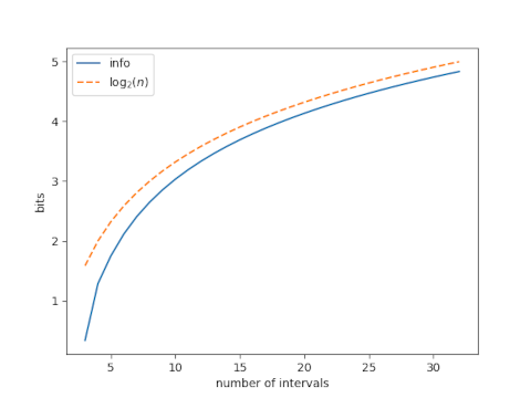
So how does the information content vary as a function of the number of bins, and how close is it to the maximum information for n bins?

Here’s a plot, with α = 0.025.

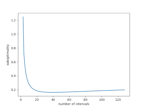
The suboptimality of our bins, i.e. the difference between log2n and the information we get from n bins, drops quickly at first as n increases, then appears to plateau.

Next lets look at just the suboptimality, and increase our range of n.

This shows that the suboptimality does not approach an asymptote but instead starts to increase. The minimum at n = 36 is 0.16 bits.

Swanson’s rule of thumb

Swanson’s rule of thumb [1] says that the mean of a moderately skewed probability distribution can be approximated by the weighted average of the 10th, 50th, and 90th percentile, with weights 0.3, 0.4, and 0.3 respectively. Because it is based on percentiles, the rule is robust to outliers. Swanson’s rule is used in the oil and gas industry, but I don’t believe it’s widely known outside of that sector.

This post will apply Swanson’s rule to three distributions to see how well it does. I’ll plot the bias in Swanson’s rule and skewness for three distributions families as the shape parameters vary.

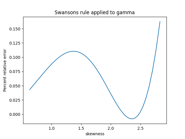
First, here’s a plot for the gamma distribution with shape parameter k varying from 0.5 to 10.

The skewness of a gamma distribution is 1/√k. So unless k is close to 0, the skewness of a gamma distribution is small and the error in Swanson’s rule is very small.

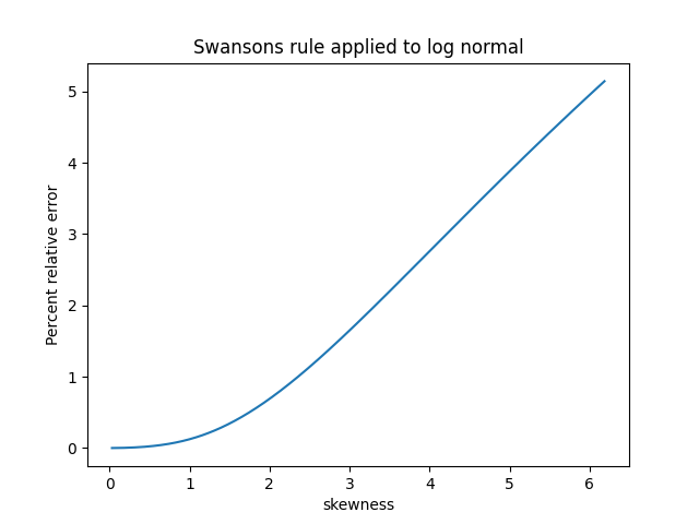
For the log normal I let the shape parameter σ vary from 0.01 to 1; I didn’t use larger parameters because skewness for the log normal increases very rapidly as a function of σ. Over the range I plotted the percentage relative error in Swanson’s rule is roughly equal to the skewness.

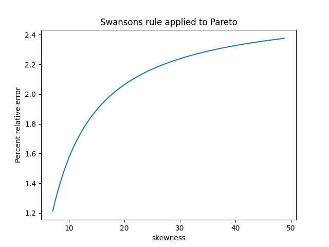
The skewness of a Pareto distribution is undefined unless the shape parameter is greater than 3. The plot below is based on shape parameters between 3.1 and 4. The skewness decreases as the shape parameter increases, asymptotically approaching 2.

Based on these examples, Swanson’s rule does indeed work pretty well when skewness is small. It works well for the gamma distribution in general because skewness is always small (unless the shape parameter k is tiny). But the log normal distribution shows that the assumption of small skewness is important.

For the Pareto distribution, Swanson’s rule works well when the shape parameter is large and the skewness is small. But this was kind of a stress test for Swanson’s rule because often the Pareto distribution is used when the skewness is large if not infinite.


[1] Swanson’s 30-40-30 rule. A. Hurst, G. C. Brown, R. I. Swanson. AAPG Bulletin, December 2000

New R book

Five years ago I recommended the book Learning Base R. Here’s the last paragraph of my review:

Now there are more books on R, and some are more approachable to non-statisticians. The most accessible one I’ve seen so far is Learning Base R by Lawrence Leemis. It gets into statistical applications of R—that is ultimately why anyone is interested in R—but it doesn’t start there. The first 40% or so of the book is devoted to basic language features, things you’re supposed to pick up by osmosis from a book focused more on statistics than on R per se. This is the book I wish I could have handed my programmers who had to pick up R.

Now there’s a second edition. The author has gone through the book and made countless changes, many of them small updates that might be unnoticeable. Here are some of the changes that would be more noticeable.

  1. There are 265 new exercises.
  2. Chapter 26 (statistics) and Chapter 28 (packages) got a complete overhaul.
  3. Dozens of new functions are introduced (either in the body of the text or through exercises).
  4. New sections include the switch function (in Chapter 13 on relational operators), algorithm development (in Chapter 23 on iteration), analysis of variance (in Chapter 26 on statistics), and time series analysis (in Chapter 26 on statistics).

I was impressed with the first edition, and the new edition promises to be even better.

The book is available at Barnes & Noble and Amazon.

Yule statistics Y and Q

I recently wrote about the Yule-Simon distribution. The same Yule, George Udny Yule, is also known for the statistics Yule’s Y and Yule’s Q. The former is also known as the coefficient of colligation, and the latter is also known as the Yule coefficient of association.

Both measure how things are related. Given a 2 × 2 contingency table

\begin{tabular} {|c|c|} \hline $a$ & $b$ \\ \hline $c$ & $d$ \\ \hline \end{tabular}

with non-negative entries, Yule’s Y is defined by

Y = \frac{\sqrt{ad} - \sqrt{bc}}{\sqrt{ad} + \sqrt{bc}}

and Yule’s Q is defined by

Q = \frac{ad - bc}{ad + bc}

Both essentially measure how much bigger ad is than bc but are weighted differently.

The algebraic properties of these two statistics may be more interesting than their statistical properties. For starters, both Y and Q produce values in the interval (−1, 1), and each is an inverse of the other:

\begin{align*} Q &= \frac{2Y}{1 + Y^2} \\ Y &= \frac{1 - \sqrt{1 = Q^2}}{Q} \end{align*}

There’s some simple but interesting algebra going on here. Define

f(x) = \frac{1-z}{1+z}

This simple function comes up surprisingly often. It’s a Möbius transformation, and it comes up in diverse applications such as designing antennas and mental math shortcuts. More on that here.

If we define

z = \frac{bc}{ad}

and

W_p = f(z^p)

then W generalizes both Q and Y: setting p = 1 gives us Q and setting p = 1/2 gives us Y.

Given the value of W with subscript p, we could easily solve for the value of W with another subscript q, analogous to solving Q for Y and Y for Q above.

W_p = f(z^p) \to^{f}{z^p} \to{x^{q/p} z^q \to^{f} f(z^q) = W_q

If you’re expecting f−1 rather than f over the first arrow, you’re right, but f is its own inverse so we could just write f instead.

Related posts

Comparing three discrete power laws

Yesterday I wrote about the zeta distribution and the Yule-Simon distribution and said that they, along with the Zipf distribution, are all discrete power laws. This post fills in detail for that statement.

The probability mass functions for the zeta, Zipf, and Yule-Simon distributions are as follows.

\begin{align*} f_\zeta(k; s) &= k^{-s} / \zeta(s) \\ f_y(k; \rho) &= \rho B(k, \rho+1) \\ f_z(k; N, s) &= k^{-s} / H_{N,s} \end{align*}

Here the subscripts ζ, y, and z stand for zeta, Yule, and Zipf respectively. The distribution parameters follow after the semicolon.

Comparing Zipf and zeta

The Zipf distribution is only defined on the first N positive integers. The normalizing constant for the Zipf distribution is the Nth generalized harmonic number with exponent s.

H_{N,s} = \sum_{k=1}^N k^{-s}

As N goes to infinity, HN,s converges to ζ(s); this is the definition of the ζ function. So the Zipf and zeta distributions are asymptotically equal.

Comparing zeta and Yule

This post showed that for large k,

f_y(k; \rho) \approx \rho \Gamma(\rho + 1) \frac{1}{(k+\rho)^{\rho + 1}}

That is, fy(k, ρ) is proportional to a power of k, except k is shifted by an amount ρ.

To compare the zeta and Yule distributions we’ll need to compare zeta with s+1 to Yule with ρ in order to make the exponents agree, and we’ll need to shift the zeta distribution by s+1.

When we plot the ratio of the pmfs, we see that the distributions agree in the limit as k gets large.

In this plot s = ρ = 1.5.

The ratio is approaching a constant, and in fact the limit is

\frac{1}{ \rho \,\Gamma(\rho + 1)\,\zeta(s+1)}

based on the ratio of the proportionality constants.

Comment

Note that the three distributions are asymptotically proportional, given the necessary shift in k, but in different ways. The Zipf distribution converges to the zeta distribution, for every k, as N goes to infinity. The zeta and Yule distributions are asymptotically proportional as k goes to infinity. So one proportion is asymptotic in a parameter N and one is asymptotic in an argument k.

Yule-Simon distribution

The Yule-Simon distribution, named after Udny Yule and Herbert Simon, is a discrete probability with pmf

f(k; \rho) = \rho B(k, \rho + 1)

The semicolon in f(k; ρ) suggests that we think of f as a function of k, with a fixed parameter ρ. The way the distribution shows the connection to the beta function, but for our purposes it will be helpful to expand this function using

B(x, y) = \frac{\Gamma(x) \, \Gamma(y)}{\Gamma(x+y)}

and so

\begin{align*} f(k; \rho) &= \rho B(k, \rho + 1) \\ &= \rho \Gamma(\rho + 1) \,\,\frac{\Gamma(k)}{\Gamma(k + \rho + 1)} \\ &= \rho \Gamma(\rho + 1) \,\, \frac{1}{(k + \rho)^{\underline{\rho + 1}}} \end{align*}

Ignore the first part of the last line, ρ Γ(ρ + 1), because it doesn’t involve k. It helps to ignore proportionality constants in probability densities when they’re not necessary. What’s left is the (ρ + 1) falling power of k + ρ.

For large values of k, the falling power term is asymptotically equal to kρ+1. To see this, let k = 1000 and ρ = 3. Then we’re saying that the ratio of

1003 × 1002 × 1001 × 1000

to

1000 × 1000 × 1000 × 1000

is approximately 1, and the ratio converges 1 as k increases.

This says that the Yule-Simon distribution is a power law in the tails, just like the Zipf distribution and the zeta distribution. Details of the comparison between these three distributions are given here.

Related posts

Mahalanobis distance and Henry V

I was reading a stats book that mentioned Mahalanobis distance and that made me think of Non Nobis from Henry V, a great scene in a great movie. As far as I know, there’s no connection between Mahalanobis and Non Nobis except that both end in “nobis.”

Since Mahalanobis is an Indian surname and Non Nobis is Latin, there’s probably no etymological connection between the two except maybe way back in Indo-European.

Mahalanobis distance is Euclidean distance adapted to a multivariate normal distribution. Specifically, the squared distance between two column vectors x and y is

(xy)T S−1 (xy)

where S is the covariance matrix for a multivariate Gaussian distribution.

You might look at this and ask why the matrix in the middle has to be the inverse of a covariance matrix. Couldn’t it be any invertible matrix? Isn’t this just Euclidean distance in transformed coordinates? Yes and yes. But Mahalanobis thought of how to use it in statistics.

Mahalanobis’ birthday, June 29, is National Statistics Day in India in his honor.

Probability of a magical permutation

Take a permutation of the numbers 1 through n² and lay out the elements of the permutation in a square. We will call a permutation a magic permutation if the corresponding square is a magic square. What is the probability that a permutation is a magic permutation? That is, if you fill a grid randomly with the numbers 1 through n², how likely are you to get a magic square?

For example, we could generate a random permutation in Python and see whether it forms a magic square.

>>> import numpy as np
>>> np.random.permutation(9).reshape(3,3)
array([[4, 7, 3],
       [2, 6, 5],
       [8, 0, 1]])

The first row adds up to 14 and the second row adds up to 13, so this isn’t a magic square. We could write a script to do this over and over and check whether the result is a magic square.

The exact number of magic squares of size n is known for n up to 5, and we have Monte Carlo estimates for larger values of n.

The number of unique magic squares, modulo rotations and reflections, of size 1 through 5 is

1, 0, 1, 880, 275305224.

For n > 2 the total number of magic squares, counting rotations and reflections as different squares, is 8 times larger than the numbers above. This is because the group of rotations and reflections of a square, D4, has 8 elements.

The probability that a permutation of the numbers 1 through 9, arranged in a square, gives a magic square is 8/9!. The corresponding probability for the numbers 1 through 16 is 8 × 880/16!, and for the numbers 1 through 25 we have 8 × 275305224/25!.

    |---+-------------|
    | n | Prob(magic) |
    |---+-------------|
    | 3 | 2.20459e-05 |
    | 4 | 3.36475e-10 |
    | 5 | 1.41990e-16 |
    |---+-------------|

It looks like the exponents are in roughly a linear progression, so maybe you could fit a line fairly well to the points on a logarithmic scale. In fact, empirical studies suggest that the probability that a permutation of the first n² positive integers is magic decreases a little faster than exponentially.

We could fit a linear regression to the logs of the numbers above to come up with an estimate for the result for n = 6. We expect the estimate could be pretty good, and likely an upper bound on the correct answer. Let’s see what actually happens with a little R code.

    > x <- c(3,4,5)
    > y <- 8*c(1/factorial(9), 880/factorial(16), 275305224/factorial(25))
    > m <- lm(log(y) ~ x)
    > predict(m, data.frame(x=c(6)))
    1
    -48.77694

This says we’d estimate that the natural log of the probability that a permutation of the first 6² positive integers is magic is -48.77694. So the estimate of the probability itself is

exp(−48.77694) = 6.55306 × 10⁻²²

We don’t know the number of magic squares of size n = 6, but the number of distinct squares has been estimated [1] at

(0.17745 ± 0.00016) × 1020

and so the total number including rotations and reflections would be 8 times higher. This says we’d expect our probability to be around

8 × 0.17745 × 1020 / 36! = 3.18162 × 10⁻²²

So our estimate is off by about a factor of 2, and as predicted it does give an upper bound.

Looking back at our regression model, the slope is -12.88 and the intercept is 28.53. This suggests that an upper bound of the probability of a permutation of size n² being magical is

exp(28.53 − 12.88 n).

In closing I’d like to point out that the estimate for n = 6 that we’re referencing above did not come from simply permuting 36 integers over and over and counting how many of the permutations correspond to magic squares. That would take far too long. It’s quite likely that after the first billion billion tries you would not have seen a magic permutation. To estimate such a small number to four significant figures requires a more sophisticated Monte Carlo procedure.

Related posts

[1] See OEIS sequence A006052
Data swamps

swamp

I recently heard the term data swamp, a humorous take on data lakes. I thought about data swamps yesterday when I hiked past the literal swamp in the photo above.

Swamps are a better metaphor than lakes for heterogeneous data collections because a lake is a homogeneous body of water. What makes a swamp a swamp is its heterogeneity.

The term “data lake” may bring up images of clear water, maybe an alpine lake like Lake Tahoe straddling California and Nevada. “Data swamp” makes me think of Louisiana’s Atchafalaya Basin, which is probably a more appropriate image for most data lakes.

Related posts

T test with unequal variances

The test statistic in the t-test does not exactly follow a Student t distribution except under ideal conditions.

If you’re comparing data from two normally distributed populations to see whether they have the same mean, the test statistic for the two-sample t-test does not have a t distribution unless the two populations have equal variance.

Robustness

Maybe this isn’t a problem. Your data didn’t exactly come from a normal distribution, so maybe it doesn’t matter that the test statistic doesn’t exactly have a t distribution. It’s a matter of robustness.

I’ve written before about the robustness of the t-test to violations of the normality assumption. In that post I assumed two populations have the same variance, but not a normal distribution. The conclusion was that departures from the normal distribution don’t matter so much, but departures from symmetry do.

For this post we’ll keep the normality assumption but have unequal variances. We know that the distribution of the test statistic is approximately, but not exactly, a t distribution. But what distribution does it have? I’ve seen it called “not pleasant” [1] but I haven’t seen a plot of it, so I’m curious.

Details

Suppose we have n samples from a random variable X and m samples from a random variable Y, and that the sample variances for the two samples are sX and sY respectively. Our test statistic for equality of the two means is

T = \frac{\bar{X} - \bar{Y}}{\sqrt{\dfrac{s_x^2}{n} + \dfrac{s_Y^2}{m}}}

Sattertwhaite’s approximation for the distribution on T is a Student t distribution with degrees of freedom equal to

\hat{\nu} = \frac{\left(\dfrac{s_X^2}{n} + \dfrac{s_Y^2}{m} \right )^2 }{\dfrac{s_X^4}{n^2(n-1)} + \dfrac{s_Y^4}{n^2(n-1)}}

This is known as the Welch-Satterthrwaite equation.

There are numerous minor variations on the two-sample t-test, and the one using degrees of freedom in the Welch-Satterthrwaite equation is known as Welch’s t-test.

Simulation

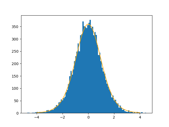
For simulation I let X be a normal random variable with mean 100 and standard deviation 1, and Y be a normal random variable with mean 100 and standard deviation 50. I drew 15 samples from X and 12 from Y and computed the statistic T. I did this 10,000 times and plotted a histogram of the values of T. The result has very nearly a t distribution.

At least in this example, any deviance from the t distribution is minor. Welch’s t-test is said to be robust to differences in variance, and this is an example of it living up to its reputation.

Related posts

[1] Casella and Berger, Statistical Inference.