Another problem with A/B testing: interaction effects

The previous post looked at a paradox with A/B testing: your final result may depend heavily on the order of your tests. This post looks at another problem with A/B testing: the inability to find interaction effects.

Suppose you’re debating between putting a photo of a car or a truck on your website, and you’re debating between whether the vehicle should be red or blue. You decide to use A/B testing, so you test whether customers prefer a red truck or a blue truck. They prefer the blue truck. Then you test whether customers prefer a blue truck or a blue car. They prefer the blue truck.

Maybe customers would prefer a red car best of all, but you didn’t test that option. By testing vehicle type and color separately, you didn’t learn about the interaction of vehicle type and color. As Andrew Gelman and Jennifer Hill put it [1],

Interactions can be important. In practice, inputs that have large main effects also tend to have large interactions with other inputs. (However, small main effects do not preclude the possibility of large interactions.)

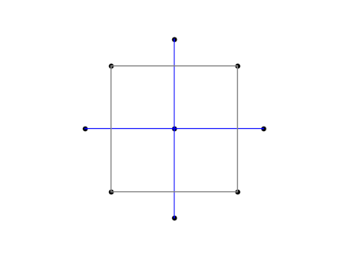
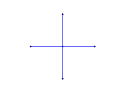
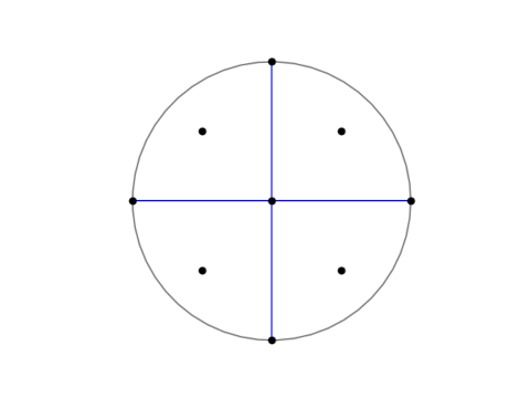
Notice that sample size is not the issue. Suppose you tested the red truck against the blue truck with 1000 users and found that 88.2% preferred the blue truck. You can be quite confident that users prefer the blue truck to the red truck. Suppose you also used 1000 users to test the blue truck against the blue car and this time 73.5% preferred the blue truck. Again you can be confident in your results. But you failed to learn something that you might have learned if you’d split 100 users between four options: red truck, blue truck, red car, blue car.

Experiment size

This is an example of a factorial design, testing all combinations of the factors involved. Factorial designs seem impractical because the number of combinations can grow very quickly as the number of factors increases. But if it’s not practical to test all combinations of 10 factors, for example, that doesn’t mean that it’s impractical to test all combinations of two factors, as in the example above. It is often practical to use a full factorial design for a moderate number of factors, and to use a fractional factorial design with more factors.

If you only test one factor at a time, you’re betting that interaction effects don’t matter. Maybe you’re right, and you can optimize your design by optimizing each variable separately. But if you’re wrong, you won’t know.

Agility

The advantage of A/B tests is that they can often be done rapidly. Blue or red? Blue. Car or truck? Truck. Done. Now let’s test something else.

If the only options were between a rapid succession of tests of one factor at a time or one big, complicated statistical test of everything, speed might win. But there’s another possibility: a rapid succession of slightly more sophisticated tests.

Suppose you have 9 factors that you’re interested in, and you understandably don’t want to test several replications of 29 = 512 possibilities. You might start out with a (fractional) factorial design of 5 of the factors. Say that only one of these factors seems to make much difference, no matter what you pair it with. Next you do another experiment testing 5 factors at a time, the winner of the first experiment and the 4 factors you haven’t tested yet. This lets you do two small experiments rather than one big one.

Note that in this example you’re assuming that the factors that didn’t matter in the first experiment wouldn’t have important interactions with the factors in the second experiment. And your assumption might be wrong. But you’re making an educated guess, based on data from the first experiment. This is less than ideal, but it’s better than the alternative of testing every factor one at a time, assuming that no interactions matter. Assuming that some interactions don’t matter, based on data, is better than making a blanket assumption that no interactions matter, based on no data.

Testing more than one factor at a time can be efficient for screening as well as for finding interactions. It can help you narrow in on the variables you need to test more thoroughly.

Related posts

[1] Andrew Gelman and Jennifer Hill. Data Analysis Using Regression and Multilevel/Hierarchical Models. Cambridge University Press, 2007.

ASQ/ANSI Z1.4 sampling procedures

I mentioned the other day that the US military standard MIL-STD-105 for statistical sampling procedures lives on in the ASQ/ANSI standard Z1.4. The Department of Defense cancelled their own standard in 1995 in favor of adopting civilian standards, in particular ASQ/ANSI Z1.4.

There are two main differences between military standard and its replacement. First, the military standard is free and the ASNI standard costs $199. Second, the ASNI standard has better typography. Otherwise the two standards are remarkably similar.

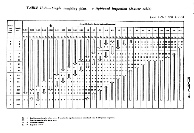
For example, the screen shot from MIL-STD-105 that I posted the other day appears verbatim in ASQ/ASNI Z1.4, except with better typesetting. The table even has the same name: “Table II-B Single sampling plans for tightened inspection (Master table).” Since the former is public domain and the latter is copyrighted, I’ll repeat my screenshot of the former.

MIL-STD-105E Table II-B

Everything I said about the substance of the military standard applies to the ASNI standard. The two give objective, checklist-friendly statistical sampling plans and acceptance criteria. The biggest strength and biggest weakness of these plans is the lack of nuance. One could create more sophisticated statistical designs that are more powerful, but then you lose the simplicity of a more regimented approach.

A company could choose to go down both paths, using more informative statistical models for internal use and reporting results from the tests dictated by standards. For example, a company could create a statistical model that takes more information into account and use it to assess the predictive probability of passing the tests required by sampling standards.

Related links

Sharing data without letting it go

Sharing data

Suppose two companies would like to share data, but they’d also each like to retain ownership of their own data. They’d like to enable querying as if each company had given the other all its data, without actually letting go of its data.

Maybe the two companies are competitors who want to collaborate for a particular project. Or maybe the companies each have data that they are not legally allowed to share with the other. Maybe one company is interested in buying (the data of) the other and would like to have some sort of preview of what they may be buying.

Differential privacy makes this possible, and can be useful even if privacy is not an issue. The two companies have data on inanimate widgets, not persons, and yet they have privacy-like concerns. They don’t want to hand over row-level data about their widgets, and yet they both want to be able to pose questions about the combined widget data. The situation is analogous to being concerned about the “privacy” of the widgets.

Both companies would deposit data with a trusted third party, and gain access to this data via an API that implements differential privacy. Such APIs let users pose queries but do not allow either side to request row-level data.

How is this possible? What if one party poses a query that unexpectedly turns out to be asking for row-level data? For example, maybe someone asks for the average net worth of customers in Alaska, assuming there are hundreds of such customers, but the data only contains one customer in Alaska. What was intended to be an aggregate query turns out to be a row-level query.

Differential privacy handles this sort of thing automatically. It adds an amount of random noise to each query in proportion to how sensitive the query is. If you ask for what amounts to data about an individual person (or individual widget) the system will add enough noise to the result to prevent revealing row-level information. (The system may also refuse to answer the query; this is done more often in practice than in theory.) But if you ask a question that reveals very little information about a single database row, the amount of noise added will be negligible.

The degree of collaboration can be limited up front by setting a privacy budget for each company. (Again, we may not necessarily be talking about the privacy of people. We may be looking at analogous protections on units of information about physical things, such as results of destructive testing of expensive hardware.)

Someone could estimate at the start of the collaboration how large the privacy budget would need to be to allow both companies to satisfy their objectives without being so large as to risk giving away intellectual property that the parties do not wish to exchange. This budget would be spent over the course of the project. When the parties exhaust their privacy budgets, they can discuss whether to allow each other more query budget.

This arrangement allows both parties the ability to ask questions of the combined data as if they had exchanged data. However, neither party has given up control of its data. They have given each other some level of information inferred from the combined data, but neither gives a single row of data to the other.

Related posts

Robustness of mean range

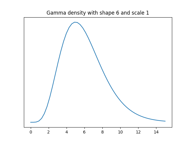
Let’s suppose we have data that comes from a distribution that is approximately normal but has a heavier right tail, specifically a gamma distribution with shape 6.

gamma(6,1) PDF

We’d like to estimate the standard deviation of the data source. If the data were normally distributed, the sample standard deviation would be the most efficient unbiased estimator. But what about this example where the data are roughly normally distributed? How well does sample standard deviation compare to the mean range? Following the convention of ANSI Z1.4 we’ll average the ranges of samples of 5.

The variance of a gamma random variable with scale 1 is equal to its shape parameter, so our data has variance 6, and so standard deviation √6. We will pretend that we don’t know this and see how well we can infer this value using random samples. We’ll compare the statistical efficiency of the mean of the ranges of k samples of 5 each and the standard deviation based on 5k samples for k = 2 and 4.

First we’ll use the following code to estimate the population standard deviation with 10 samples two ways: with sample standard deviation and with the average of the range of two samples of 5. We’ll take the absolute value of the difference between each estimate and the true value, and repeat this 1,000 times to simulate the mean absolute error.

    from scipy.stats import gamma, t
    
    def meanrange(y, k):
        scale = 0.430 # scale factor for n=5
        s = 0
        for i in range(k):
            sample = y[5*i:5*(i+1)]
            s += max(sample) - min(sample)
        return scale*s/k
    
    n = 5
    k = 2
    shape = 6
    sigma = shape**0.5
    
    stderr = 0
    mrerr = 0
    N = 1000
    for _ in range(N):
        y = gamma(shape).rvs(size=n*k)    
        std = y.std(ddof=1)
        mr = meanrange(y, k)
        stderr += abs(std-sigma)
        mrerr += abs(mr-sigma)
    print(stderr/N, mrerr/N)    

The mean absolute error was 0.532 using sample standard deviation and 0.550 using mean range.

When I changed k to 4, the mean absolute error using the sample standard deviation was 0.377. The mean absolute error using the range of 4 samples of 5 each time was 0.402.

The error in both methods was comparable, though the sample standard deviation did slightly better.

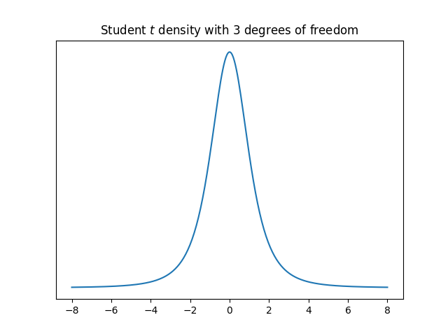
Next I repeated the experiment drawing samples from a Student t distribution with 3 degrees of freedom, a distribution with heavy tails.

PDF of a t distribution with nu = 3

When k = 2, the mean absolute errors were 0.603 and 0.574 for sample standard deviation and mean range respectively. When k = 4, the errors were 0.484 and 0.431. Again the errors are comparable, but this time the mean range was more accurate.

Related posts

Using mean range method to measure variability

The most common way to measure variability, at least for data coming from a normal distribution, is standard deviation. Another less common approach is to use mean range. Standard deviation is mathematically simple but operationally a little complicated. Mean range, on the other hand, is complicated to analyze mathematically but operationally very simple.

ASQ/ANSI Z1.9

The ASQ/ANSI Z1.9 standard, Sampling Procedures and Table for Inspection by Variables for Percent Nonconforming, gives several options for measuring variability, and one of these is the mean range method. Specifically, several samples of five items each are drawn, and the average of the ranges is the variability estimate. The ANSI Z1.9 standard grew out of, and is still very similar to, the US military standard MIL-STD-414 from 1957. The ANSI standard, last updated in 2018, is not that different from the military standard from six decades earlier.

The average mean is obviously simple to carry out: take five samples, subtract the smallest value from the largest, and write that down. Repeat this a few times and average the numbers you wrote down. No squares, no square roots, easy to carry out manually. This was obviously a benefit in 1957, but not as much now that computers are ubiquitous. The more important advantage today is that the mean range can be more robust for heavy-tailed data. More on that here.

Probability distribution

The distribution of the range of a sample is not simple to write down, even when the samples come from a normal distribution. There are nice asymptotic formulas for the range as the number of samples goes to infinity, but five is a bit far from infinity [1].

This is a problem that was thoroughly studied decades ago. The random variable obtained by averaging k ranges from samples of n elements each is denoted

\overline{W}_{n,k}

or sometimes without the subscripts.

Approximate distribution

There are several useful approximations for the distribution of this statistic. Pearson [2] evaluated several proposed approximations and found that the best one for n < 10 (as it is in our case, with n = 5) to be

\frac{\overline{W}}{\sigma} \approx \frac{c \chi_\nu}{\sqrt{\nu}}

Here σ is the standard deviation of the population being sampled, and the values of c and ν vary with n and k. For example, when n = 5 and k = 4, the value of ν is 14.7 and the value of c is 2.37. The value of c doesn’t change much as k gets larger, though the value of ν does [3].

Note that the approximating distribution is chi, not the more familiar chi square. (I won’t forget a bug I had to chase down years ago that was the result of seeing χ in a paper and reading it as χ². Double, triple, quadruple check, everything looks right. Oh wait …)

For particular values of n and k you could use the approximate distribution to find how to scale mean range to a comparable standard deviation, and to assess the relative efficiency of the two methods of measuring variation. The ANSI/ASQ Z1.9 standard gives tables for acceptance based on mean range, but doesn’t go into statistical details.

Related posts

[1] Of course every finite number is far from infinity. But the behavior at some numbers is quite close to the behavior at infinity. Asymptotic estimates are not just an academic exercise. They can give very useful approximations for finite inputs—that’s why people study them—sometimes even for inputs as small as five.

[2] E. S. Pearson (1952) Comparison of two approximations to the distribution of the range in small samples from normal populations. Biometrika 39, 130–6.

[3] H. A. David (1970). Order Statistics. John Wiley and Sons.

Military Standard 105

Military Standard 105 (MIL-STD-105) is the grand daddy of sampling acceptance standards. The standard grew out of work done at Bell Labs in the 1930s and was first published during WWII. There were five updates to the standard, the last edition being MIL-STD-105E, published in 1989.

In 1995 the standard was officially cancelled when the military decided to go with civilian quality standards moving forward. Military Standard 105 lives on through its progeny, such as ANSI/ASQ Z1.4, ASTM E2234, and ISO 2859-1. There’s been an interesting interaction between civilian and military standards: Civilian organizations adopted military standards, then the military adopted civilian standards (which evolved from military standards).

From a statistical perspective, it seems a little odd that sampling procedures are given without as much context as an experiment designed from scratch might have. But obviously a large organization, certainly an army, must have standardized procedures. A procurement department cannot review thousands of boutique experiment designs the way a cancer center reviews sui generis clinical trial designs. They have to have objective procedures that do not require a statistician to evaluate.

MIL-STD-105E Table II-B

Of course manufacturers need objective standards too. The benefits of standardization outweigh the potential benefits of customization: economic efficiency trumps the increase in statistical efficiency that might be obtained from a custom sampling approach.

Although the guidelines in MIL-STD-105 are objective, they’re also flexible. For example, instead of dictating a single set of testing procedures, the standard gives normal, tightened, and reduced procedures. The level of testing can go up or down based on experience. During normal inspection, if two out of five consecutive lots have been rejected, then testing switches to tightened procedures. Then after five consecutive lots have been accepted, normal testing can resume. And if certain conditions are met under normal procedures, the manufacturer can relax to reduced procedures [1]. The procedures are adaptive, but there are explicit rules for doing the adapting.

This is very similar to my experience with adaptive clinical trial designs. Researchers often think that “adaptive” means flying by the seat of your pants, making subjective decisions as a trial progresses. But an adaptive statistical design is still a statistical design. The conduct of the experiment may change over time, but only according to objective statistical criteria set out in advance.

MIL-STD-105 grew out of the work of smart people, such as Harold Dodge at Bell Labs, thinking carefully about the consequences of the procedures. Although the procedures have all the statistical lingo stripped away—do this thing this many times, rather than looking at χ² values—statistical thought went into creating these procedures.

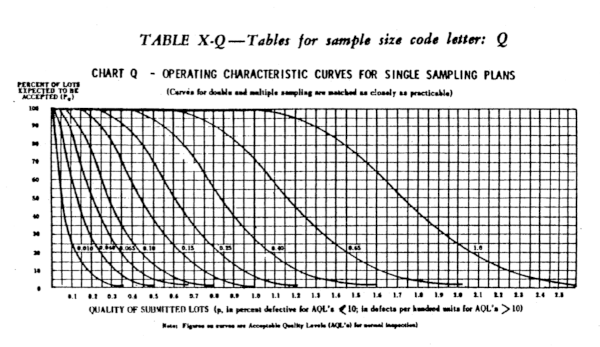
MIL-STD-105E Table X Q

Related links

[1] This isn’t the most statistically powerful approach because it throws away information. It only considers whether batches met an acceptance standard; it doesn’t use the data on how many units passed or failed. The units in one batch are not interchangeable with units in another batch, but neither are they unrelated. A more sophisticated approach might use a hierarchical model that captured units within batches. But as stated earlier, you can’t have someone in procurement review hierarchical statistical analyses; you need simple rules.

Using Python as a statistical calculator

This post is for someone unfamiliar with SciPy who wants to use Python to do basic statistical calculations. More specifically, this post will look at working with common families of random variables—normal, exponential, gamma, etc.—and how to calculate probabilities with these.

All the statistical functions you need will be in the stats subpackage of SciPy. You could import everything with

    >>> from scipy.stats import *

This will make software developers cringe because it’s good software development practice to only import what you need [1]. But we’re not writing software here; we’re using Python as a calculator.

Distributions

Every distribution in SciPy has a location parameter loc which defaults to 0, and scale parameter scale that defaults to 1.

The table below lists additional parameters that some common distributions have.

Distribution SciPy name    Parameters
normal norm
exponential expon
beta beta shape1, shape2
binomial binom size, prob
chi-squared chi2 df
F f df1, df2
gamma gamma shape
hypergeometric hypergeom M, n, N
Poisson poisson lambda
Student t t df

When using any statistical software its good to verify that the software is using the parameterization that you expect. For example, the exponential distribution can be parameterized by rate or by scale. SciPy does everything by scale. One way to test the parameterization is to calculate the mean. For example, if the mean of an exp(100) random variable is 100, you’re software is using the scale paraemterization. If the mean is 1/100, it’s using the rate.

Functions

For a random variable X from one of the families above, we’ll show how to compute Prob(Xx), Prob(Xx), and how to solve for x given one of these probabilities. And for discrete distributions, we’ll show how to find Prob(X = p).

CDF: Cumulative distribution function

The probability Prob(Xx) is the CDF of X at x. For example, the probability that a standard normal random variable is less than 2 is

    norm.cdf(2)

We didn’t have to specify the location or scale because the standard normal uses default parameters. If X had mean 3 and standard deviation 10 we’d call

    norm.cdf(2, loc=3, scale=10)

For another example, suppose we’re working with a gamma distribution with shape 3 and scale 5 and want to know the probability of such a random variable taking on a value less than 2. Then we’d call

    gamma.cdf(2, 3, scale=5)

The second argument, 2, is the shape parameter.

CCDF: Complementary cumulative distribution function

The probability Prob(Xx) is the complementary CDF of X at x, which is 1 minus the CDF at x. SciPy uses the name sf for the CCDF. Here “sf” stands for survival function.

Why have both a CDF and CCDF function? One reason is convenience, but a more important reason is numerical accuracy. If a probability p is very near 1, then 1 – p will be partially or completely inaccurate.

For example, let X be a standard normal random variable. The probability that X is greater than 9 is

    norm.sf(9)

which is on the order of 10−19. But if we compute

    1 - norm.cdf(9)

we get exactly 0. Floating point numbers have 16 figures of precision, and we need 19 to represent the difference between our probability and 1. More on why mathematical libraries have functions that seem unnecessary at first here.

Inverse CDF

SciPy calls the inverse CDF function ppf for percentile point function.

For example, suppose X is a gamma random variable with shape 3 and scale 5, and we want to solve for the value of x such that Prob(Xx) is 0.7. We could do this with

    gamma.ppf(0.7, 3, scale=5)

Inverse CCDF

SciPy calls the inverse CCDF function isf for inverse survival function. So, for example,

    gamma.isf(0.3, 3, scale=5)

should return the same value as the example above because the point where the right tail has probability 0.3 is the same as the point where the left tail has probability 0.7.

Probability mass function

For a discrete random variable X we can compute the probability mass function, the probability that X takes on a value x. Unsurprisingly SciPy calls this function pmf.

For example, the probability of seeing 6 heads out of 10 flips of a fair coin is computed by

    binom.pmf(6, 10, 0.5)

Getting help

To find out more about a probability distribution, call help with that distribution as an argument. For example, you could call

    help(hypergeom)

to read more about the hypergeometric distribution.

For much more information, including topics not addressed here, see the documentation for scipy.stats.

***

[1] The reason to not import more than you need is to reduce namespace confusion. If you see a function foo, is that the foo function from package A or from package B. The most common way this comes up in statistics is confusion over the gamma function and the gamma distribution. In SciPy, the gamma function is in scipy.special while the gamma distribution is in scipy.stats. If you’ve imported everything from scipy.stats then gamma means scipy.stats.gamma. You could bring the gamma function into your environment by importing it with another name. For example

    from scipy.special import gamma as gammaf

would import the gamma function giving it the name gammaf.

Save big money on big queries

server room

I was surprised the first time a client told me that a query would cost them $100,000 to run. If you think about querying a database on your laptop, a long query would take a minute, and what’s the cost of a minute’s worth of electricity? Too small to meter.

But some of my clients have a LOT of data. (Some also come to me with spreadsheets of data.) If you have billions of records hosted in a cloud database like Snowflake, the cost of a query isn’t negligible, especially if it involves complex joins.

There are three ways to reduce the cost of expensive queries.

First of all, it may be possible to solve a different way the problem you’re trying to solve with the expensive query. Maybe the query is the most direct approach but there’s a more economical indirect approach.

Second, it may be possible to rewrite the query into a logically equivalent query that runs faster.

Third, it may be possible to save a tremendous amount of money by tolerating a small probability of error. For example, you may be able to use reservoir sampling rather than an exhaustive query.

This last approach is often misunderstood. Why would you tolerate any chance of error when you could have the exact answer? One reason is that the exact answer might cost 1000x as much to obtain. More importantly, the “exact” result may be the exact answer to a query that is trying estimate something else. The probability of error induced by random sampling may be small relative to the probability of error intrinsic in the problem being solved.

If you’d like me to take a look at how I could reduce your query costs, let’s talk.

Related posts

Efficiently testing a black box

Suppose you have a black box that takes three bits as input and produces one bit as output. You could think of the input bits as positions of toggle switches, and the output bit as a light attached to the box that is either on or off.

Full factorial design

Now suppose that only one combination of 3 bits produces a successful output. There’s one way to set the switches that makes the light turn on. You can find the successful input by brute force if you test all 2³ = 8 possible inputs. In statistical lingo, you are conducting an experiment with a factorial design, i.e. you test all combinations of inputs.

See the Python code below for a text version of this design

In the chart above, each row is an experimental run and each column is a bit. I used − and + rather than 0 and 1 because it is conventional in this topic to use a minus sign to indicate that a factor is not present and a plus sign to indicate that it is present.

Fractional factorial design

Now suppose your black box takes 4 bits as inputs, but only 3 of them matter. One of the bits does nothing, but you don’t know which bit that is. You could use a factorial design again, testing all 24 = 16 possible inputs. But there’s a more clever approach that requires only 8 guesses. In statistical jargon, this is a fractional factorial design.

See the Python code below for a text version of this design

No matter which three bits the output depends on, all combinations of those three bits will be tested. Said another way, if you delete any one of the four columns, the remaining columns contain all combinations of those bits.

Replications

Now suppose your black box takes 8 bits. Again only 3 bits matter, but you don’t know which 3. How many runs do you need to do to be certain of finding the successful combination of 3 bits? It’s clear that you need at least 8 runs: if you know that the first three bits are the important ones, for example, you still need 8 runs. And it’s also clear that you could go back to brute force and try all 28 = 256 possible inputs, but the example above raises your hopes that you could get by with less than 256 runs. Could you still get by with 8? That’s too much to hope for, but you could use only 16 runs.

--------, +----+++, -+--+-++, ++--++--, --+-+++-, +-+-+--+, -++--+-+, +++---+-, ---+++-+, +--++-+-, -+-+-++-, ++-+---+, --++--++, +-++-+--, -++++---, ++++++++

Note that since this design works for 8 factors, it also works for fewer factors. If you had 5, 6, or 7 factors, you could use the first 5, 6, or 7 columns of the design above.

This design has some redundancy: every combination of three particular bits is tested twice. This is unfortunate in our setting because we are assuming the black box is deterministic: the right combination of switches will always turn the light on. But what if the right combination of switches probably turns on the light? Then redundancy is a good thing. If there’s an 80% chance that the right combination will work, then there’s a 96% chance that at least one of the two tests of the right combination will work.

Fractional factorial experiment designs are usually used with the assumption that there are random effects, and so redundancy is a good thing.

You want to test each main effect, i.e. each single bit, and interaction effects, i.e. combinations of bits, such as pairs of bits or triples of bits. But you assume that not all possible interactions are important; otherwise you’d need a full factorial design. You typically hit diminishing returns with interactions quickly: pairs of effects are often important, combinations of three effects are less common, and rarely would an experiment consider fourth order interactions.

If only main effects and pairs of main effects matter, and you have a moderately large number of factors n, a fractional factorial design can let you use a lot less than 2n runs while giving you as many replications of main and interaction effects as you want.

Verification

The following Python code verifies that the designs above have the claimed properties.

    import numpy as np
    from itertools import combinations
    
    def verify(matrix, k):
        "verify that every choice of k columns has 2^k unique rows"
        nrows, ncols = matrix.shape
        for (a, b, c) in combinations(range(ncols), k):
            s = set()
            for r in range(nrows):
                s.add((matrix[r,a], matrix[r,b], matrix[r,c]))
            if len(s) != 2**k:
                print("problem with columns", a, b, c)
                print("number of unique elements: ", len(s))
                print("should be", 2**k)
                return
        print("pass")
    
    m = [
        [-1, -1, -1, -1],
        [-1, -1, +1, +1],
        [-1, +1, -1, +1],
        [-1, +1, +1, -1],
        [+1, -1, -1, +1],
        [+1, -1, +1, -1],
        [+1, +1, -1, -1],
        [+1, +1, +1, +1]
    ]
    
    verify(np.matrix(m), 3)
    
    m = [
        [-1, -1, -1, -1, -1, -1, -1, -1],
        [+1, -1, -1, -1, -1, +1, +1, +1],
        [-1, +1, -1, -1, +1, -1, +1, +1],
        [+1, +1, -1, -1, +1, +1, -1, -1],
        [-1, -1, +1, -1, +1, +1, +1, -1],
        [+1, -1, +1, -1, +1, -1, -1, +1],
        [-1, +1, +1, -1, -1, +1, -1, +1],
        [+1, +1, +1, -1, -1, -1, +1, -1],
        [-1, -1, -1, +1, +1, +1, -1, +1],
        [+1, -1, -1, +1, +1, -1, +1, -1],
        [-1, +1, -1, +1, -1, +1, +1, -1],
        [+1, +1, -1, +1, -1, -1, -1, +1],
        [-1, -1, +1, +1, -1, -1, +1, +1],
        [+1, -1, +1, +1, -1, +1, -1, -1],
        [-1, +1, +1, +1, +1, -1, -1, -1],
        [+1, +1, +1, +1, +1, +1, +1, +1],
    ]
    
    verify(np.matrix(m), 3)

Related services

Regex to match ICD-11 code

ICD codes are diagnostic codes created by the WHO. (Three TLAs in just the opening paragraph!)

The latest version, ICD-11, went into effect in January of this year. A few countries are using ICD-11 now; it’s expected to be at least a couple years before the US moves from ICD-10 to ICD-11. (I still see ICD-9 data even though ICD-10 came out in 1994.)

One way that ICD-11 codes differ from ICD-10 codes is that the new codes do not use the letters I or O in order to prevent possible confusion with the digits 1 and 0. In the code below, “alphabetic” and “alphanumeric” implicitly exclude the letters I and O.

Another way the codes differ is the that the second character in an ICD-10 is a digit whereas the second character in an ICD-11 code is a letter.

What follows is a heavily-commented regular expression for matching ICD-11 codes, along with a few tests to show that the regex matches things it should and does not match things it should not.

Of course you could verify an ICD-11 code by searching against an exhaustive list of such codes, but the following is much simpler and may match some false positives. However, it is future-proof against false negatives: ICD-11 codes added in the future will conform to the pattern in the regular expression.

import re

icd11_re = re.compile(r"""
    ^                  # beginning of string
    [A-HJ-NP-Z0-9]     # alphanumeric
    [A-HJ-NP-Z]        # alphabetic
    [0-9]              # digit
    [A-HJ-NP-Z0-9]     # alphanumeric
    ((\.               # optional starting with .
    [A-HJ-NP-Z0-9])    # alphanumeric
    [A-HJ-NP-Z0-9]?)?  # optional further refinement
    $                  # end of string
    """, re.VERBOSE)

good = [
    "ND52",   # fracture of arm, level unspecified
    "9D00.3", # presbyopia
    "8B60.Y", # other specified increased intercranial pressure
    "DB98.7Z" # portal hypertension, unspecified
]

bad = [
    "ABCD",    # third character must be digit
    "AB3D.",   # dot must be followed by alphanumeric
    "9D0O.3",  # letter 'O' should be number 0
    "DB9872",  # missing dot
    "AB3",     # too short
    "DB90.123" # too long
]

for g in good:
    assert(icd11_re.match(g))
for b in bad:
    assert(icd11_re.match(b) == None)

Related posts