Wire gauge and user perspective

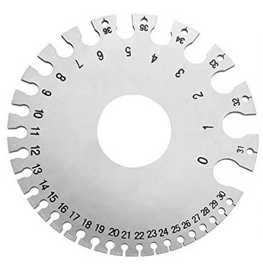
wire gauge measurement device

Wire gauge is a perennial source of confusion: larger numbers denote smaller wires. The reason is that gauge numbers were assigned from the perspective of the manufacturing process. Thinner wires require more steps in production. This is a common error in user interface design and business more generally: describing things from your perspective rather than from the customer’s perspective.

Restaurants

When you order food at a restaurant, the person taking your order may rearrange your words before repeating them back to you. The reason may be that they’re restating it in manufacturing order, the order in which the person preparing the food needs the information.

Rheostats

A rheostat is a device for controlling resistance in an electrical circuit. It would seem natural for an engineer to give a user a control to vary resistance in Ohms. But Ohm’s law says

V = IR,

i.e. voltage equals current times resistance. Users expect that when they turn a knob clockwise they get more of something—brighter lights, louder music, etc.—and that means more voltage or more current, which means less resistance. Asking users to control resistance reverses expectations.

If I remember correctly, someone designed a defibrillator once where a knob controlled resistance rather than current. If that didn’t lead to someone dying, it easily could have.

Research

When I worked for MD Anderson Cancer Center, I managed the development of software for clinical trial design and conduct. Our software started out very statistician-centric and became more user-centric. This was a win, even for statisticians.

The general pattern was to move from eliciting technical parameters to eliciting desired behavior. Tell us how you want the design to behave and we’ll solve for the parameters to make that happen. Sometimes we weren’t able to completely automate parameter selection, but we were at least able to give the user a head start in knowing where to look.

Relax

Technical people don’t always want to have their technical hat on. Sometimes they want to relax and be consumers. When statisticians wanted to crank out a clinical trial design, they wanted software that was easy to use rather than technically transparent. That’s the backstory to this post.

It’s generally a good idea to conceal technical details, but provide a “service panel” to expose details when necessary.

Related posts

How to put a series in hypergeometric form

I skipped a step in the previous post, not showing how a series was put into the form of a hypergeometric function.

Actually I skipped two steps. I first said that a series was not obviously hypergeometric, and yet at first glance it sorta is.

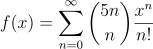
I’d like to make up for both of these omissions, but with a simpler example. It looks like a hypergeometric series, and it is, but it’s not the one you might think. The example will be the function below.

f(x)  = \sum_{n=0}^\infty \binom{5n}{n} \frac{x^n}{n!}

Rising powers

Hypergeometric functions are defined by series whose coefficients are rising powers.

The nth rising power of a is

(a)n = a (a+1) (a + 2) … (a + n – 1).

More on rising powers here. The coefficient of xn in a series defining a hypergeometric function is a ratio of nth rising powers of constants.

Why the example isn’t obvious

You can write factorials as rising powers: n! = (1)n. The binomial coefficient in our example is a ratio of rising powers:

(5n)! = (1)5n

in the numerator and

n! (4n)! = (1)n (1)4n

in the denominator. So why aren’t we done? Because although these are all rising powers, they’re not all nth rising powers. The subscripts on the (a)n are all different: 5n, 4n, and n.

So is our function not hypergeometric? It is, but we’ll have to introduce more parameters.

Rational polynomials

Another way to define hypergeometric series is to say that the ratio of consecutive coefficients is a rational function of the index n. This is very succinct, but not as explicit as the definition in terms of rising powers, though they’re equivalent.

In addition to brevity, this definition has another advantage: the hypergeometric parameters are the negatives of the zeros and poles of said rational function. The zeros are the upper parameters and the poles are the lower parameters.

This is how you put a series in hypergeometric form, if it has such a form. It’s also how you test whether a series is hypergeometric: a series is hypergeometric if and only if the ratio of consecutive terms is a single rational function of the index.

Back to our example

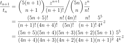
The ratio of the (n+1)st term to the nth term in our series is

\begin{align*} \frac{t_{n+1}}{t_n} &= \left.\binom{5(n+1)}{n+1} \frac{z^{n+1}}{(n+1)!} \middle/{\binom{5n}{n}} \frac{z^n}{n!} \right. \\ &= \frac{(5n+5)!}{(n+1)! \,(4n+4)!} \,\frac{n!\,(4n)!}{(5n)!} \, \frac{n!}{(n+1)!}\frac{5^5}{4^4} z\\ &= \frac{(5n+5)(5n+4)(5n+3)(5n+2)(5n+1)}{(4n+4)(4n+3)(4n+2)(4n+1)(n+1)^2} \, \frac{5^5}{4^4} z \end{align*}

and the final expression is a rational function of n. We can read the hypergeometric function parameters directly from this rational function. The upper parameters are 1, 4/5, 3/5, 2/5, and 1/5. The lower parameters are 1, 3/4, 2/4, 1/4, and 1. Identical factors in the upper and lower parameters cancel each other out, so we can remove the 1 from the list of upper parameters and remove one of the 1’s from the list of lower parameters [1].

So our example function is

{}_4 F_4\left(\frac{1}{5}, \frac{2}{5}, \frac{3}{5}, \frac{4}{5};\,\, \frac{1}{4}, \frac{1}{2}, \frac{3}{4}, 1; \,\,\frac{3125}{256}x \right)

The order of the upper parameters doesn’t matter, and neither does the order of the lower parameters, though it matters very much which ones are upstairs and which are downstairs. The subscript to the left of the F gives the number of upper parameters and the subscript to the right gives the number of lower parameters. These subscripts are redundant since you could just count the number of parameters between the semicolons, but they make it easier to tell at a glance what class of hypergeometric function you’re working with.

Spot check

Let’s evaluate our original series and our hypergeometric series at a point to make sure they agree. I chose x = 0.01 to stay within the radius of convergence of the hypergeometric series.

Both

    Sum[Binomial[5 n, n] (0.01^n)/n!, {n, 0, Infinity}]

and

    HypergeometricPFQ[
        {1/5, 2/5, 3/5, 4/5}, 
        {1/4, 2/4, 3/4, 1},
        0.01*3125/256]

return the same value, namely 1.05233.

Related posts

[1] The extra factor of n! in the denominator of hypergeometric functions complicates things. It seems like an unfortunately historical artifact to me, but maybe it’s a net benefit for reasons I’m not thinking of. When we look at zeros of the numerator and denominator, we have a single 1 on top and three ones on bottom. The 1 on top cancels out one of the 1s on bottom, but why don’t we have two 1s in the lower parameters? Because one of them corresponds to the extra n! in the denominator.

Quintic trinomial root

This post looks at an exercise from Special Functions, exercise 6 in Appendix E.

Suppose that xm+1 + axb = 0. Show that

x = \frac{b}{a} - \frac{b^{m+1}}{a^{m+2}} + \frac{2m + 2}{2!} \frac{b^{2m+1}}{a^{2m+3}} - \frac{(3m+2)(3m+3)}{3!} \frac{b^{3m+1}}{a^{3m+4}} + \cdots

Use this formula to find a solution to x5 + 4x + 2 = 0 to four decimal places of accuracy. When m = 0 this series reduces to the geometric series. Write this sum as a hypergeometric series.

There are several things I find interesting about this exercise.

  • It’s a possibly useful result.
  • It’s an application of Lagrange’s inversion formula; that’s where the series comes from.
  • The equation has m+1 roots. What’s special about the root given by the series?
  • The sum is not obviously hypergeometric.
  • What happens when the sum diverges? Is it a useful asymptotic series? Does the analytic continuation work?

I want to address the last two points in this post. Maybe I’ll go back and address the others in the future. To simplify things a little, I will assume m = 4.

The parameters of the hypergeometric series are not apparent from the expression above, nor is it even apparent how many parameters you need. It turns out you need m upper parameters and m-1 lower parameters. Since we’re interested in m = 4, that means we have a hypergeometric function of the form 4F3.

x = \frac{b}{a}\,\, {}_4 F_3\left(\frac{1}{5},\frac{2}{5},\frac{3}{5},\frac{4}{5};\frac{1}{2}, \frac{3}{4}, \frac{5}{4} ; -\frac{3125b^4}{256a^5}\right)

We can evaluate this expression in Mathematica as

    f[a_, b_] := (b/a) HypergeometricPFQ[
        {1/5, 2/5, 3/5, 4/5}, 
        {1/2, 3/4, 5/4}, 
        -3125 b^4 / (256 a^5)
    ]

When we evaluate f[4, -2] we get -0.492739, which is the only real root of

x5 + 4x + 2 = 0.

Recall that the sign on b is negative, so we call our function with b = -2.

Now lets, try another example, solving for a root of

x5 + 3x − 4 = 0.

If we plug a = 3 and b = 4 into the series at the top of the post, the series diverges immediately, not giving a useful asymptotic series before it diverges.

The series defining our hypergeometric function diverges for |z| > 1, and we’re evaluating it at z = −3125/243. However, the function can be extended beyond the unit disk by analytic continuation, and when we ask Mathematica to numerically evaluate the root with by running

    N{ f[3, 4] ]

we get 1, which is clearly a root of x5 + 3x − 4.

Related posts

Theory, practice, and integration

Theory and practice are both important. As Donald Knuth put it,

If you find that you’re spending almost all your time on theory, start turning some attention to practical things; it will improve your theories. If you find that you’re spending almost all your time on practice, start turning some attention to theoretical things; it will improve your practice.

However, there’s an implicit third factor: integration.

We can have theoretical knowledge and practical experience, but keep them isolated in different parts of our brain. It’s possible to do well in a probability class, and play poker well, but not be able to think about probability while playing poker, to be no better at poker for having taken probability.

It may not be immediately obvious that someone excels at integration. It comes out in off-the-cuff remarks, little comments that show someone can quickly apply abstract theory to a concrete problem.

It’s hard to teach integration. A course can have lectures and labs, but that doesn’t mean students will fully connect the two in their minds. Maybe the connection forms later after some experience and some contemplation.

Information loss and entropy

John Baez, Tobias Fritz, and Tom Leinster wrote a nice paper [1] that shows Shannon entropy is the only measure of information loss that acts as you’d expect, assuming of course you have the right expectations. See their paper for all the heavy lifting. All I offer here is an informal rewording of the hypotheses.

The authors say that

We show that Shannon entropy gives the only concept of information loss that is functorial, convex-linear and continuous.

You could reword this by saying

Shannon entropy is the only measure of information loss that composes well, mixes well, and is robust.

Saying that a measure of information loss composes well means that the information lost by doing two processes f and then g is the sum of the information lost by doing f and the information lost by doing g. This is what the authors describe as functorial.

When I refer to something mixing well, I have in mind mixtures in the sense of probability. A mixture is a random choice of random variables, such as flipping a coin to decide which of two dice to roll.

Going back to our two processes f and g, if we choose to do f with probability p and to do g with probability (1 – p) then the information loss from this mixture process should be p times the information loss from f plus (1-p) times the information lost from g. Instead of saying this mixes well, you could say it behaves as expected, where “as expected” is a pun on expected value. The authors describe this as convex-linear because the expected information loss is a convex combination of the two possible losses.

Robustness is a more colloquial term for continuity. Something is robust if small changes in inputs should lead to small changes in outputs. If you make this statement rigorous, you end up with the definition of continuity. If we change a process f a little then we should change our measure of information loss a little.

More on information theory

[1] A characterization of entropy in terms of information loss. On arXiv.

Partition symmetry

Let p(M, N, n) be the number of partitions of the integer n into at most M parts, each containing integers at most N. Then

p(M, N, n) = p(N, M, n).

That is, you can swap the size of the partition multisets and the upper bound on the elements in the multisets.

For example, lets look at the partitions of 6 into multisets with at most 3 elements. The Mathematica command

    IntegerPartitions[6, 3]

returns

  • {6}
  • {5, 1}
  • {4, 2}
  • {4, 1, 1}
  • {3, 3}
  • {3, 2, 1}
  • {2, 2, 2}

Now let’s look at the partitions of 6 into sets with any number of elements, but with no elements greater than 3. The Mathematica command

    IntegerPartitions[6, All, {1, 2, 3}]

returns

  • {3, 3}
  • {3, 2, 1}
  • {3, 1, 1, 1}
  • {2, 2, 2}
  • {2, 2, 1, 1}
  • {2, 1, 1, 1, 1}
  • {1, 1, 1, 1, 1, 1}}

Both return a list of 7 multisets because

p(3, 6, 6) = p(6, 3, 6) = 7.

As another example, let’s look at partitions of 11. First we look at partitions with at most 3 elements, with each element less than or equal to 5. We list these with

    IntegerPartitions[11, 3, Range[5]]

which gives

  • {5, 5, 1}
  • {5, 4, 2}
  • {5, 3, 3}
  • {4, 4, 3}

Now let’s look at partitions of 11 into multisets with at most 5 elements, each less than or equal to 3 using

    IntegerPartitions[11, 5,  Range[3]]

This gives us

  • {5, 5, 1}
  • {5, 4, 2}
  • {5, 3, 3}
  • {4, 4, 3}

Not only do both lists have the same number of partitions, which we would expect because

p(3, 5, 11) = p(5, 3, 11),

in this case they actually give the same list of partitions.

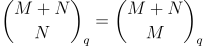
The symmetry relation here follows from the symmetry of the q-binomial coefficient because p(M, N, n) equals the coefficient of qn in the q-binomial

\binom{M+N}{N}_q = \binom{M+N}{M}_q

It’s not immediately obvious from the definition that the rational function defining q-binomial coefficient is in fact a polynomial, but it is.

More partition posts

Numbering the branches of the Lambert W function

The previous post used the Lambert W function to solve an equation that came up in counting partitions of an integer. The first solution found didn’t make sense in context, but another solution, one on a different branch, did. The default branch k = 0 wasn’t what we were after, but the branch k = -1 was.

Branches 0 and -1

The branch corresponding to k = 0 is the principal branch. In mathematical notation, the k is usually a subscript, i.e W0(z) is the principal branch of the Lambert W function. For real z ≥ -1/e it returns a real value. It’s often what you want, and that’s why it’s the default in software implementations such as SciPy and Mathematica. More on that below.

The only other branch that returns real values for real inputs is W−1 which returns real values for -1/ez < 0.

If you’re working strictly with real numbers, you only need to be concerned with branches 0 and -1. If branch 0 doesn’t give you what you expect, try branch -1, if your argument is negative.

SciPy and Mathematica

SciPy implements Wk with lambertw(z). The parameter k defaults to 0.

The Mathematica function ProductLog[z] implements W0(z), and ProductLog[k, z] implements Wk.

Note that Mathematica and Python list their arguments in opposite orders.

Branch numbering

The branches are numbered in order of their imaginary parts. That is, The imaginary part of Wk (z) is an increasing function of k. For example, here is a list of the numerical values of the imaginary parts of Wk (1) for k running from -3 to 3.

    Table[N[Im[ProductLog[k, 1]]], {k, -3, 3}]
    {-17.1135, -10.7763, -4.37519, 0., 4.37519, 10.7763, 17.1135}

Note the zero in the middle because W0(1) is real.

Recovering k

Given z and a value Wk (z) with k unknown, you can determine k with

k = \frac{W_k(z) + \log W_k(z) - \log z}{2\pi i}

with the exception that if the expression above is 0 and -1/ez < 0 then k = -1. See [1].

For example, let z = 1 + 2i and w = W3 (z).

    z = 1 + 2 I
    w = ProductLog[3, z]

Now pretend you don’t know how w was computed. When you compute

    N[(w + Log[w] - Log[z])/(2 Pi I)]

the result is 3.

Partition example

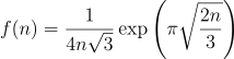
The discussion of the W function here grew out of a problem with partitions. Specifically, we wanted to solve for n such that
f(n) = \frac{1}{4n\sqrt{3}} \exp\left( \pi \sqrt{\frac{2n}{3}} \right)

is approximately a trillion. We found in the previous post that solutions of the equation

a w^b \exp(c w^d) = x

are given by

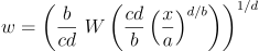
w = \left(\frac{b}{cd} \,\,W\left(\frac{cd}{b} \left(\frac{x}{a} \right )^{d/b} \right )\right )^{1/d}

Our partition problem corresponds to a = 1/√48, b = -1, c = π √(2/3), and d = 1/2. We found that the solution we were after came from the k = -1 branch.

    N[( (b/(c d)) ProductLog[-1, (x/a)^(d/b) c d /b])^(1/d)]
    183.852

Even though our final value was real, the intermediate values were not. The invocation of W−1 in the middle returns a complex value:

    N[ProductLog[-1, ((x/a)^(d/b) c d /b)^(1/d)]]
    -32.5568 - 3.24081 I

We weren’t careful about specifying ranges and branch cuts, but just sorta bulldozed our way to a solution. But it worked: it’s easy to verify that 183.852 is the solution we were after.

***

[1] Unwinding the branches of the Lambert W function by Jeffrey, Hare, and Corless. The Mathematical Scientist 21, 1&ndash;7 (1996)

Solving equations with Lambert’s W function

In the previous post we wanted to find a value of n such that f(n) = 1012 where

f(n) = \frac{1}{4n\sqrt{3}} \exp\left( \pi \sqrt{\frac{2n}{3}} \right)

and we took a rough guess n = 200. Turns out f(200) ≈ 4 × 10¹² and that was good enough for our purposes. But what if we wanted to solve f(n) = x accurately?

We will work our way up to solving f(n) = 1012 exactly using the Lambert W function.

Lambert’s W function

If you can solve one equation involving exponential functions you can bootstrap your solution solve a lot more equations.

The Lambert W function is defined to be the function W(x) that maps each x to a solution of the equation

w exp(w) = x.

This function is implemented Python under scipy.special.lambertw. Let’s see how we could use it solve similar equations to the one that define it.

Basic bootstrapping

Given a constant c we can solve

cw exp(w) = x

simply by solving

w exp(w) = x/c,

which says w = W(x/c).

And we can solve

w exp(cw) = x

by setting y = cw and solving

y exp(y) = cx.

and so cw = W(cx) and w = W(cx)/c.

Combining the two approaches above shows that the solution to

aw exp(bw) = x

is

w = W(bx/a) / b.

We can solve

exp(w) / w = x

by taking the reciprocal of both sides and applying the result above with a = 1 and b = -1.

More generally, we can solve

wc exp(w) = x

by raising both sides to the power 1/c; the reciprocal the special case c = 1.

Similarly, we can solve

w exp(wc) = x

by setting y = wc , changing the problem to

y−1/c exp(y) = x.

Putting it all together

We’ve now found how to deal with constants and exponents on w, inside and outside the exponential function. We now have all the elements to solve our original problem.

We can solve the general equation

a w^b \exp(c w^d) = x

with

w = \left(\frac{b}{cd} \,\,W\left(\frac{cd}{b} \left(\frac{x}{a} \right )^{d/b} \right )\right )^{1/d}

The equation at the top of the post corresponds to a = 1/√48, b = -1, c = π √(2/3), and d = 1/2.

We can code this up in Python as follows.

    from scipy.special import lambertw

    def soln(a, b, c, d, x):
        t = (x/a)**(d/b) *c*d/b
        return (lambertw(t)*b/(c*d))**(1/d) 

We can verify that our solution really is a solution by running it though

    from numpy import exp, pi

    def f(a, b, c, d, w):
        return a*w**b * exp(c*w**d)

to make sure we get our x back.

When we run

    a = 0.25*3**-0.5
    b = -1
    c = pi*(2/3)**0.5
    d = 0.5
    x = 10**12

    w = soln(a, b, c, d, x)
    print(f(a, b, c, d, w))

we do indeed get x back.

    a = 0.25*3**-0.5
    b = -1
    c = pi*(2/3)**0.5
    d = 0.5

    w = soln(a, b, c, d, 10)
    print(f(a, b, c, d, w))

When we take a look at the solution w, we get 1.443377079584187e-13. In other words, we get a number near zero. But our initial guess was w = 200. What went wrong?

Nothing went wrong. We got a solution to our equation. It just wasn’t the solution we expected.

The Lambert W function has multiple branches when viewed as a function on complex numbers. It turns out the solution we were expecting is on the branch SciPy denotes with k = -1. If we add this to the call to lambertw above we get the solution 183.85249773880142 which is more in line with what we expected.

More Lambert W posts

Estimating the number of integer partitions

Last week I wrote a few posts that included code that iterated over all partitions of a positive integer n. See here, here, and here. How long would it take these programs to run for large n?

For this post, I’ll focus just on how many partitions there are. It’s interesting to think about how you would generate the partitions, but that’s a topic for another time.

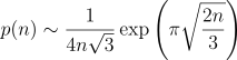
Ramanujan discovered an asymptotic formula for p(n), the number of partitions of n. As n increases,

p(n) \sim \frac{1}{4n\sqrt{3}} \exp\left( \pi \sqrt{\frac{2n}{3}} \right)

The ratio of the two sides of the equation goes to 1 as n → ∞, but how accurate is it for the sizes of n that you might want to iterate over in a program?

Before answering that, we need to decide what range of n we might use. Let’s be generous and say we might want to look at up to a trillion (1012) partitions. How big of a value of n does that correspond to? The estimate above shows p(200) is on the order of 4 × 10¹², so we only need to be concerned with n ≤ 200. (See the next post for how to exactly solve for a n that gives a specified value.)

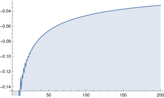
Here’s a plot to show the relative error in the approximation above.

Here’s the Mathematica code that made the plot.

    approx[n_] := Exp[Pi Sqrt[2 n/3]]/(4 n Sqrt[3])
    DiscretePlot[ 1 - approx[n]/PartitionsP[n], {n, 200}]

So the estimate above is always an under-estimate, at least about 4% low over the range we care about. It’s good enough for a quick calculation. It tells us, for example, to be very patient if we’re going to run any program that needs to iterate over all partitions of an integer even as small as 100.

The function PartitionsP above returns the number of partitions in its argument. It returned quickly, so it certainly did not generate all partitions and count them. Algorithms for computing p(n) might make an interesting blog post another time.

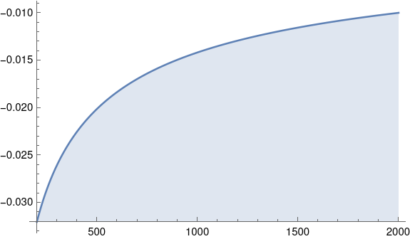
Even though it would be impractical to iterate over the partitions of larger values, we still might be curious what the plot above looks like for larger arguments. Let’s see what the plot would look like for n between 200 and 2000.

The shape of the curve is practically the same.

The relative error dropped by about a factor or 3 when we increased n by a factor of 10. So we’d expect if we increase n by another factor of 10, the relative error would drop about another factor of 3, and indeed that’s what happens: when n = 20,000, the relative error is about -0.003.