What is a confidence interval?

At first glance, a confidence interval is simple. If we say [3, 4] is a 95% confidence interval for a parameter θ, then there’s a 95% chance that θ is between 3 and 4. That explanation is not correct, but it works better in practice than in theory.

If you’re a Bayesian, the explanation above is correct if you change the terminology from “confidence” interval to “credible” interval. But if you’re a frequentist, you can’t make probability statements about parameters.

Confidence intervals take some delicate explanation. I took a look at Andrew Gelman and Deborah Nolan’s book Teaching Statistics: a bag of tricks,  to see what they had to say about teaching confidence intervals. They begin their section on the topic by saying “Confidence intervals are complicated …” That made me feel better. Some folks with more experience teaching statistics also find this challenging to teach. And according to The Lady Testing Tea, confidence intervals were controversial when they were first introduced.

From a frequentist perspective, confidence intervals are random, parameters are not, exactly the opposite of what everyone naturally thinks. You can’t talk about the probability that θ is in an interval because θ isn’t random. But in that case, what good is a confidence interval? As L. J. Savage once said,

The only use I know for a confidence interval is to have confidence in it.

In practice, people don’t go too wrong using the popular but technically incorrect notion of a confidence interval. Frequentist confidence intervals often approximate Bayesian credibility intervals; the frequentist approach is more useful in practice than in theory.

It’s interesting to see a sort of détente between frequentist and Bayesian statisticians. Some frequentists say that the Bayesian interpretation of statistics is nonsense, but the methods these crazy Bayesians come up with often have good frequentist properties. And some Bayesians say that frequentist methods, such as confidence intervals, are useful because they can come up with results that often approximate Bayesian results.

Cost-benefit analysis versus benefit-only analysis

Hardly anyone cares about statistics directly. People more often care about decisions they need to make with the help of statistics. This suggests that the statistics and decision-making process should be explicitly integrated. The name for this integrated approach is “decision theory.” Problems in decision theory are set up with the goal of maximizing “utility,” the benefit you expect to get from a decision. Equivalently, problems are set up to minimize expected cost. Cost may be a literal monetary cost, but it could be some other measure of something you want to avoid.

I was at a conference this morning where David Draper gave an excellent talk entitled Bayesian Decision Theory in Biostatistics: the Utility of Utility.  Draper presented an example of selecting variables for a statistical model. But instead of just selecting the most important variables in a purely statistical sense, he factored in the cost of collecting each variable. So if two variables make nearly equal contributions to a model, for example, the procedure would give preference to the variable that is cheaper to collect. In short, Draper recommended a cost-benefit analysis rather than the typical (statistical) benefit-only analysis. Very reasonable.

Why don’t people always take this approach? One reason is that it’s hard to assign utilities to outcomes. Dollar costs are often easy to account for, but it can be much harder to assign values to benefits. For example, you have to ask “Benefit for whom?” In a medical context, do you want to maximize the benefit to patients? Doctors? Insurance companies? Tax payers? Regulators? Statisticians? If you want to maximize some combination of these factors, how do you weight the interests of the various parties?

Assigning utilities is hard work, and you can never make everyone happy. No matter how good of a job you do, someone will criticize you. Nearly everyone agrees in the abstract that considering utilities is the way to go, but in practice it is hardly ever done. Anyone who proposes a way to quantify utility is immediately shot down by people who have a better idea. The net result is that rather than using a reasonable but  imperfect idea of utility, no utility is used at all. Or rather no explicit definition of utility is used. There is usually some implicit idea of utility, chosen for mathematical convenience, and that one wins by default. In general, people much prefer to leave utilities implicit.

In the Q&A after his talk, Draper said something to the effect that the status quo persists for a very good reason: thinking is hard work, and it opens you up to criticism.

The probability that Shakespeare wrote a play

Some people object to asking about the probability that Shakespeare wrote this or that play. One objection is that someone has already written the play, either Shakespeare or someone else. If Shakespeare wrote it, then the probability is one that he did. Otherwise the probability is zero. By this reasoning, no one can make probability statements about anything that has already happened. Another objection is that probability only applies to random processes. We cannot apply probability to questions about document authorship because documents are not random.

I just ran across a blog post by Ted Dunning that weighs in on this question. He writes

The statement “It cannot be probability …” is essentially a tautology. It should read, “We cannot use the word probability to describe our state of knowledge because we have implicitly accepted the assumption that probability cannot be used to describe our state of knowledge”.

He goes on to explain that if we think about statements of knowledge in terms of probabilities, we get a consistent system, so we might as well reason as if it’s OK to use probability theory.

The uncertainty about the authorship of the play does not exist in history — an omniscient historian would know who wrote it. Nor does it exist in nature — the play was not created by a random process. The uncertainty is in our heads. We don’t know who wrote it. But if we use numbers to represent our uncertainty, and we agree to certain common-sense axioms about how this should be done, we inevitably get probability theory.

As E. T. Jaynes once put it, “probabilities do not describe reality — only our information about reality.”

Three math diagrams

Here are three pages containing diagrams that each summarize several theorems.

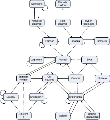
The distribution relationships page summarizing around 40 relationships between around 20 statistical distributions.

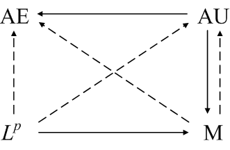
The modes of convergence page has three diagrams like the following that explain when one kind of convergence implies another: almost everywhere, almost uniform, Lp, and convergence in measure.

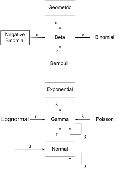
The page conjugate prior relationships is similar to the probability distribution page, but concentrates on relationships in Bayesian statistics.

What are some of your favorite diagrams? Do you have any suggestions for diagrams that you’d like to see someone make?

Random inequalities VII: three or more variables

The previous posts in this series have looked at P(X > Y), the probability that a sample from a random variable X is greater than a sample from an independent random variable Y. In applications, X and Y have different distributions but come from the same distribution family.

Sometimes applications require computing P(X > max(Y, Z)). For example, an adaptively randomized trial of three treatments may be designed to assign a treatment with probability equal to the probability that that treatment has the best response. In a trial with a binary outcome, the variables X, Y, and Z may be beta random variables representing the probability of response. In a trial with a time-to-event outcome, the variables might be gamma random variables representing survival time.

Sometimes we’re interested in the opposite inequality, P(X < min(Y,Z)). This would be the case if we thought in terms of failures rather than responses, or wanted to minimize the time to a desirable event rather than maximizing the time to an undesirable event.

The maximum and minimum inequalities are related by the following equation:

P(X < min(Y, Z)) = P(X > max(Y, Z)) + 1 − P(X > Y) − P(X > Z).

These inequalities are used for safety monitoring rules as well as to determine randomization probabilities. In a trial seeking to maximize responses, a treatment arm X might be dropped if P(X > max(Y,Z)) becomes too small.

In principle one could design an adaptively randomized trial with n treatment arms for any n ≥ 2 based on

P(X1 > max(X2, …, Xn)).

In practice, the most common value of n by far is 2. Sometimes n is 3. I’m not familiar with an adaptively randomized trial with more than three arms. I’ve heard of an adaptively randomized trial that was designed with five arms, but I don’t believe the trial ran.

Computing P(X1 > max(X2, …, Xn)) by numerical integration becomes more difficult as n increases. For large n, simulation may be more efficient than integration. Computing P(X1 > max(X2, …, Xn)) for gamma random variables with n=3 was unacceptably slow in a previous version of our adaptive randomization software. The search for a faster algorithm lead to this paper: Numerical Evaluation of Gamma Inequalities.

Previous posts on random inequalities:

How much do you expect to learn from that experiment?

Bayesian statisticians often talk about models “learning” as data accumulate. Here’s an example that applies information theory to quantify how much you can learn from an experiment using the same likelihood function but two different priors: a conjugate prior and a robust prior.

Here’s an example from a paper Luis Pericchi and I wrote recently. Suppose X ~ Normal(θ, 1) where the prior on θ is either a standard Cauchy distribution or a normal distribution with mean 0 and variance 2.19. (The variance on the normal was chosen following an example by Jim Berger so that both priors put half their mass on the interval [−1, 1].)

The expected information gain from a single observation using the normal (conjugate) prior was 0.58. The corresponding gain for the Cauchy (robust) prior was 1.20. Because robust priors are more responsive to data, the expected gain in information is larger (in this case twice as large) when using these priors.

Related: Quantifying information content

Stopping trials of ineffective drugs earlier

Valen Johnson and I recently posted a working paper on a method for stopping trials of ineffective drugs earlier. For Bayesians, we argue that our method is more consistently Bayesian than other methods in common use. For frequentists, we show that our method has better frequentist operating characteristics than the most commonly used safety monitoring method.

The paper looks at binary and time-to-event trials. The results are most dramatic for the time-to-event analog of the Thall-Simon method, the Thall-Wooten method, as shown below.

This graph plots the probability of concluding that an experimental treatment is inferior when simulating from true mean survival times ranging from 2 to 12 months. The trial is designed to test a null hypothesis of 6 months mean survival against an alternative hypothesis of 8 months mean survival. When the true mean survival time is less than the alternative hypothesis of 8 months, the Bayes factor design is more likely to stop early. And when the true mean survival time is greater than the alternative hypothesis, the Bayes factor method is less likely to stop early.

The Bayes factor method also outperforms the Thall-Simon method for monitoring single-arm trials with binary outcomes. The Bayes factor method stops more often when it should and less often when it should not. However, the difference in operating characteristics is not as pronounced as in the time-to-event case.

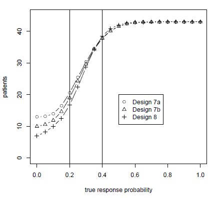
The paper also compares the Bayes factor method to the frequentist mainstay, the Simon two-stage design. Because the Bayes factor method uses continuous monitoring, the method is able to use fewer patients while maintaining the type I and type II error rates of the Simon design as illustrated in the graph below.

bayes factor vs simon two-stage designs

The graph above plots the number of patients used in a trial testing a null hypothesis of a 0.2 response rate against an alternative of a 0.4 response rate. Design 8 is the Bayes factor method advocated in the paper. Designs 7a and 7b are variations on the Simon two-stage design. The horizontal axis gives the true probabilities of response. We simulated true probabilities of response varying from 0 to 1 in increments of 0.05. The vertical axis gives the number of patients treated before the trial was stopped. When the true probability of response is less than the alternative hypothesis, the Bayes factor method treats fewer patients. When the true probability of response is better than the alternative hypothesis, the Bayes factor method treats slightly more patients.

Design 7a is the strict interpretation of the Simon method: one interim look at the data and another analysis at the end of the trial. Design 7b is the Simon method as implemented in practice, stopping when the criteria for continuing cannot be met at the next analysis. (For example, if the design says to stop if there are three or fewer responses out of the first 15 patients, then the method would stop after the 12th patient if there have been no responses.) In either case, the Bayes factor method uses fewer patients. The rejection probability curves, not shown here, show that the Bayes factor method matches (actually, slightly improves upon) the type I and type II error rates for the Simon two-stage design.

Related: Adaptive clinical trial design

Random inequalities V: beta distributions

I’ve put a lot of effort into writing software for evaluating random inequality probabilities with beta distributions because such inequalities come up quite often in application. For example, beta inequalities are at the heart of the Thall-Simon method for monitoring single-arm trials and adaptively randomized trials with binary endpoints.

It’s not easy to evaluate P(X > Y) accurately and efficiently when X and Y are independent random variables. I’ve seen several attempts that were either inaccurate or slow, including a few attempts on my part. Efficiency is important because this calculation is often in the inner loop of a simulation study. Part of the difficulty is that the calculation depends on four parameters and no single algorithm will work well for all parameter combinations.

Let g(a, b, c, d) equal P(X > Y) where X ~ beta(a, b) and Y ~ beta(c, d). Then the function g has several symmetries.

  • g(a, b, c, d) = 1 − g(c, d, a, b)
  • g(a, b, c, d) = g(d, c, b, a)
  • g(a, b, c, d) = g(d, b, c, a)

The first two relations were published by W. R. Thompson in 1933, but as far as I know the third relation first appeared in this technical report in 2003.

For special values of the parameters, the function g(a, b, c, d) can be computed in closed form. Some of these special cases are when

  • one of the four parameters is an integer
  • a + b + c + d = 1
  • a + b = c + d = 1.

The function g(a, b, c, d) also satisfies several recurrence relations that make it possible to bootstrap the latter two special cases into more results. Define the beta function

B(a, b) = Γ(a, b)/(Γ(a) Γ(b))

as usual and define

h(a, b, c, d) as B(a+c, b+d)/( B(a, b) B(c, d) ).

Then the following recurrence relations hold.

  • g(a+1, b, c, d) = g(a, b, c, d) + h(a, b, c, d)/a
  • g(a, b+1, c, d) = g(a, b, c, d) – h(a, b, c, d)/b
  • g(a, b, c+1, d) = g(a, b, c, d) – h(a, b, c, d)/c
  • g(a, b, c, d+1) = g(a, b, c, d) + h(a, b, c, d)/d

For more information about beta inequalities, see these papers:

Previous posts on random inequalities:

Subjecting fewer patients to ineffective treatments

Tomorrow morning I’m giving a talk on how to subject fewer patients to ineffective treatment in clinical trials. I should have used something like the title of this post as the title of my talk, but instead my talk is called “Clinical Trial Monitoring With Bayesian Hypothesis Testing.” Classic sales mistake: emphasizing features rather than benefits. But the talk is at a statistical conference, so maybe the feature-oriented title isn’t so bad.

Ethical concerns are the main consideration that makes biostatistics a separate branch of statistics. You can’t test experimental drugs on people the way you test experimental fertilizers on crops. In human trials, you want to stop the trial early if it looks like the experimental treatment is not as effective as a comparable established treatment, but you want to keep going if it looks like the new treatment might be better. You need to establish rules before the trial starts that quantify exactly what it means to look like a treatment is doing better or worse than another treatment. There are a lot of ways of doing this quantification, and some work better than others. Within its context (single-arm phase II trials with binary or time-to-event endpoints) the method I’m presenting stops ineffective trials sooner than the methods we compare it to while stopping no more often in situations where you’d want the trial to continue.

If you’re not familiar with statistics, this may sound strange. Why not always stop when a treatment is worse and never stop when it’s better? Because you never know with certainty that one treatment is better than another. The more patients you test, the more sure you can be of your decision, but some uncertainty always remains. So you face a trade-off between being more confident of your conclusion and experimenting on more patients. If you think a drug is bad, you don’t want to treat thousands more patients with it in order to be extra confident that it’s bad, so you stop. But you run the risk of shutting down a trial of a treatment that really is an improvement but by chance appeared to be worse at the time you made the decision to stop. Statistics is all about such trade-offs.

Related: Adaptive clinical trial design