In grad school I specialized in differential equations, but never worked with delay-differential equations, equations specifying that a solution depends not only on its derivatives but also on the state of the function at a previous time. The first time I worked with a delay-differential equation would come a couple decades later when I did some modeling work for a pharmaceutical company.
Large delays can change the qualitative behavior of a differential equation, but it seems plausible that sufficiently small delays should not. This is correct, and we will show just how small “sufficiently small” is in a simple special case. We’ll look at the equation
x′(t) = a x(t) + b x(t − τ)
where the coefficients a and b are non-zero real constants and the delay τ is a positive constant. Then [1] proves that the equation above has the same qualitative behavior as the same equation with the delay removed, i.e. with τ = 0, provided τ is small enough. Here “small enough” means
−1/e < bτ exp(−aτ) < e
and
aτ < 1.
There is a further hypothesis for the theorem cited above, a technical condition that holds on a nowhere dense set. The solution to a first order delay-differential like the one we’re looking at here is not determined by an initial condition x(0) = x0 alone. We have to specify the solution over the interval [−τ, 0]. This can be any function of t, subject only to a technical condition that holds on a nowhere-dense set of initial conditions. See [1] for details.
Example
Let’s look at a specific example,
x′(t) = −3 x(t) + 2 x(t − τ)
with the initial condition x(1) = 1. If there were no delay term τ, the solution would be x(t) = exp(1 − t). In this case the solution monotonically decays to zero.
The theorem above says we should expect the same behavior as long as
−1/e < 2τ exp(3τ) < e
which holds as long as τ < 0.404218.
Let’s solve our equation for the case τ = 0.4 using Mathematica.
tau = 0.4
solution = NDSolveValue[
    {x'[t] == -3 x[t] + 2 x[t - tau], x[t /; t <= 1] == t },
    x, {t, 0, 10}]
Plot[solution[t], {t, 0, 10}, PlotRange -> All]
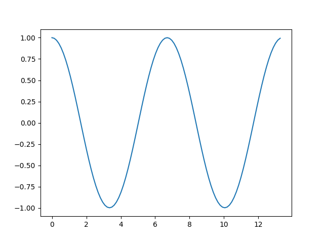
This produces the following plot.
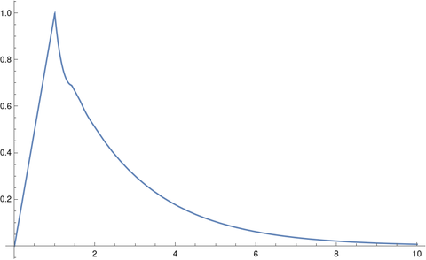
The solution initially ramps up to 1, because that’s what we specified, but it seems that eventually the solution monotonically decays to 0, just as when τ = 0.
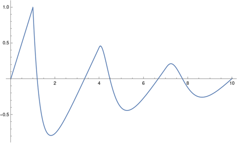
When we change the delay to τ = 3 and rerun the code we get oscillations.
[1] R. D. Driver, D. W. Sasser, M. L. Slater. The Equation x’ (t) = ax (t) + bx (t – τ) with “Small” Delay. The American Mathematical Monthly, Vol. 80, No. 9 (Nov., 1973), pp. 990–995