Integration by Darts

Posted on 1 April 2015 by John

dartboard

Monte Carlo integration has been called “Integration by Darts,” a clever pun on “integration by parts.” I ran across the phrase looking at some slides by Brian Hayes, but apparently it’s been around a while. The explanation that Monte Carlo is “integration by darts” is fine as a 0th order explanation, but it can be misleading.

Introductory courses explain Monte Carlo integration as follows.

Plot the function you want to integrate.
Draw a box that contains the graph.
Throw darts (random points) at the box.
Count the proportion of darts that land between the graph and the horizontal axis.
Estimate the area under the graph by multiplying the area of the box by the proportion above.

In principle this is correct, but this is far from how Monte Carlo integration is usually done in practice.

For one thing, Monte Carlo integration is seldom used to integrate functions of one variable. Instead, it is mostly used on functions of many variables, maybe hundreds or thousands of variables. This is because more efficient methods exist for low-dimensional integrals, but very high dimensional integrals can usually only be computed using Monte Carlo or some variation like quasi-Monte Carlo.

If you draw a box around your integrand, especially in high dimensions, it may be that nearly all your darts fall outside the region you’re interested in. For example, suppose you throw a billion darts and none land inside the volume determined by your integration problem. Then the point estimate for your integral is 0. Assuming the true value of the integral is positive, the relative error in your estimate is 100%. You’ll need a lot more than a billion darts to get an accurate estimate. But is this example realistic? Absolutely. Nearly all the volume of a high-dimensional cube is in the “corners” and so putting a box around your integrand is naive. (I’ll elaborate on this below. [1])

So how do you implement Monte Carlo integration in practice? The next step up in sophistication is to use “importance sampling.” [2] Conceptually you’re still throwing darts at a box, but not with a uniform distribution. You find a probability distribution that approximately matches your integrand, and throw darts according to that distribution. The better the fit, the more efficient the importance sampler. You could think of naive importance sampling as using a uniform distribution as the importance sampler. It’s usually not hard to find an importance sampler much better than that. The importance sampler is so named because it concentrates more samples in the important regions.

Importance sampling isn’t the last word in Monte Carlo integration, but it’s a huge improvement over naive Monte Carlo.

***

[1] So what does it mean to say most of the volume of a high-dimensional cube is in the corners? Suppose you have an n-dimensional cube that runs from −1 to 1 in each dimension and you have a ball of radius 1 inside the cube. To make the example a little simpler, assume n is even, n = 2k. Then the volume of the cube is 4^k and the volume of the sphere is π^k / k!. If k = 1 (n = 2) then the sphere (circle in this case) takes up π/4 of the volume (area), about 79%. But when k = 100 (n = 200), the ball takes up 3.46×10⁻¹⁶⁹ of the volume of the cube. You could never generate enough random samples from the cube to ever hope to land a single point inside the ball.

[2] In a nutshell, importance sampling replaces the problem of integrating f(x) with that of integrating (f(x) / g(x)) g(x) where g(x) is the importance sampler, a probability density. Then the integral of (f(x) / g(x)) g(x) is the expected value of (f(X) / g(X)) where X is a random variable with density given by the importance sampler. It’s often a good idea to use an importance sampler with slightly heavier tails than the original integrand.

Integration trick

Posted on 22 October 2014 by John

Here’s a clever example from Paul Nahin’s new book Inside Interesting Integrals. Suppose you want to evaluate

$\int_{-1}^1 \frac{\cos(x)}{\exp(1/x) + 1}\,dx$

Since the range of integration is symmetric around zero, you might think to see whether the integrand is an odd function, in which case the integral would be zero. (More on such symmetry tricks here.) Unfortunately, the integrand is not odd, so that trick doesn’t work directly. However, it does help indirectly.

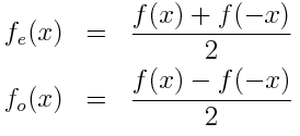
You can split any function f(x) into its even and odd parts.

$f_e(x) = \frac{f(x) + f(-x)}{2} \\ f_o(x) = \frac{f(x) - f(-x)}{2}$

The integral of a function over a symmetric interval is the integral of its even part because its odd part integrates to zero. The even part of the integrand above works out to be simply cos(x)/2 and so the integral evaluates to sin(1).

How Lp spaces nest

Posted on 11 November 2012 by John

A function f(x) is said to be in L^p if the integral of |f(x)|^p is finite. So if you know f is in L^p for some value of p, can conclude that f is also in L^q for some q? In general, no. But for two important special cases, yes. The special cases have to do with the domain of f.

If f is a function on a finite measure space and p > q, then every function in L^p is in L^q. In particular probability spaces are finite measure spaces, and so if a random variable’s pth moment exists, the qth moment exists.

If the domain of f is the integers with counting measure, f is a sequence and the “integral” of |f(x)|^p is simply a sum. Now the relationship between L^p spaces is reversed: p > q, every sequence in L^q is in L^p.

There are two reasons a function could fail to be in L^p: singularities and fat tails. In a finite measure space, there are no tails; you only have to worry about singularities. On the integers, there are no singularities; you only have to worry about tails.

Now consider functions on the whole real line. Membership in L^p says nothing about membership in L^q because now you can have singularities and fat tails.

Avoiding underflow in Bayesian computations

Posted on 26 July 2012 by John

Here’s a common problem that arises in Bayesian computation. Everything works just fine until you have more data than you’ve seen before. Then suddenly you start getting infinite, NaN, or otherwise strange results. This post explains what might be wrong and how to fix it.

A posterior density is (proportional to) a likelihood function times a prior distribution. The likelihood function is a product. The number of data points is the number of terms in the product. If these numbers are less than 1, and you multiply enough of them together, the result will be too small to represent in a floating point number and your calculation will underflow to zero. Then subsequent operations with this number, such as dividing it by another number that has also underflowed to zero, may produce an infinite or NaN result.

The instinctive reaction regarding underflow or overflow is to use logs. And often that works. If you wanted to know where the maximum of the posterior density occurs, you could find the maximum of the logarithm of the posterior density. But in Bayesian computations you often need to integrate the posterior density times some functions. Now you cannot just work with logs because logs and integrals don’t commute.

One way around the problem is to multiply the integrand by a constant so large that there is no danger of underflow. Multiplying by constants does commute with integration.

So suppose your integrand is on the order of 10^−400, far below the smallest representable number. Do you need extended precision arithmetic? No, you just need to understand your problem.

If you multiply your integrand by 10^400 before integrating, then your integrand is roughly 1 in magnitude. Then do you integration, and remember that the result is 10^400 times the actual value.

You could take the following steps.

Find m, the maximum of the log of the integrand.
Let I be the integral of exp( log of the integrand − m ).
Keep track that your actual integral is exp(m) I, or that its log is m + log I.

Note that you can be extremely sloppy in this process. You don’t need an accurate estimate of the maximum of the integrand per se. If you’re within a few dozen orders of magnitude, for example, that could be sufficient to carry out your integration without underflow.

One way to estimate the maximum is to use a frequentist estimator of your parameters as an approximate MLE, and assume that this is approximately where your posterior density takes on its maximum value. This might actually be very accurate, but it doesn’t need to be.

Note also that it’s OK if some of the evaluations of your integrand underflow to zero. You just don’t want the entire integral to underflow to zero. Places where the integrand is many orders of magnitude less than its maximum don’t contribute to the integration anyway. (It’s important that your integration pays attention to the region where the integrand is largest. A naive integration could entirely miss the most important region and completely underestimate the integral. But that’s a matter for another blog post.)

Fractional integration

Posted on 5 April 2012 by John

Define the integration operator I by

$(I,f)(x) = \int_a^x f(t)\, dt$

so I f is an antiderivative of f.

Define the second antiderivative I₂ by applying I to f twice:

$(I_2, f)(x) = \int_a^x \int_a^t f(t_1)\, dt_1\, dt$

It turns out that

$(I_2, f)(x) = \int_a^x (x - t) \, f(t)\, dt$

To see this, notice that both expressions for I₂ are equal when x = a, and they have the same derivative, so they must be equal everywhere.

Now define I₃ by applying I to I₂ and so forth defining I_n for all positive integers n. Then one can show that the nth antiderivative is given by

$(I_n, f)(x) = \frac{1}{\Gamma(n)} \int_a^x (x - t)^{n-1} \, f(t)\, dt$

The right side of this equation makes sense for non-integer values of n, and so we can take it as a definition of fractional integrals when n is not an integer.

Related post: Fractional derivatives

Numerical integration trick

Posted on 21 March 2012 by John

Suppose you want to evaluate the following integral:

$\int_{30}^\infty \exp\left( -\frac{100}{x+6} \right) \, \frac{1}{x^3} \, \dx$

We’d like to do a change of variables to make the range of integration finite, and we’d like the transformed integral to be easy to evaluate numerically.

The change of variables t = 1/x² transforms the range of integration from (30, ∞) to (0, 1/900). I’ll explain where this choice came from and why it results in a nice function to integrate.

The integrand is essentially 1/x³ for large x because the exponential term approaches 1. If the integrand were exactly 1/x³ then the change of variables t = 1/x² would make the integrand constant. So we’d expect this change of variables to give us an integrand that behaves well. In particular, the integral should be bounded at 0.

(If you’re not careful, a change of variables may just swap one kind of improper integral for another. That is, you can make the domain of integration finite, but at the cost of introducing a singularity in the transformed integrand. However, we don’t have that problem here because our change of variables was just right.)

In general, if you need to integrate a function that behaves like 1/xⁿ as x goes to infinity, try the change of variables t = 1/xⁿ⁻¹.

Related post: The care and treatment of singularities

SciPy integration misunderstanding

Posted on 20 March 2012 by John

Today I needed to compute an integral similar to this:

$\int_{1000}^\infty \frac{dx}{100, x^3}$

I used the following SciPy code to compute the integral:

from scipy.integrate import quad

def f(x):
    return 0.01*x**-3

integral, error = quad(f, 1000, sp.inf, epsrel = 1e-6)
print integral, error

My intention was to compute the integral to 6 significant figures. (epsrel is a shortened form of epsilon relative, i.e. relative error.) To my surprise, the estimated error was larger than the value of the integral. Specifically, the integral was computed as 5.15 × 10⁻⁹ and the error estimate was 9.07 × 10⁻⁹.

What went wrong? The integration routine quad lets you specify either a desired bound on your absolute error (epsabs) or a desired bound on your relative error (epsrel). I assumed that since I specified the relative error, the integration would stop when the relative error requirement was met. But that’s not how it works.

The quad function has default values for both epsabs and epsrel.

def quad(... epsabs=1.49e-8, epsrel=1.49e-8, ...):

I thought that since I did not specify an absolute error bound, the bound was not effective, or equivalently, that the absolute error target was 0. But no! It was as if I’d set the absolute error bound to 1.49 × 10⁻⁸. Because my integral is small (the exact value is 5 × 10⁻⁹) the absolute error requirement is satisfied before the relative error requirement and so the integration stops too soon.

The solution is to specify an absolute error target of zero. This condition cannot be satisfied, and so the relative error target will determine when the integration stops.

integral, error = quad(f, 1000, sp.inf, epsrel = 1e-6, epsabs = 0)

This correctly computes the integral as 5 × 10⁻⁹ and estimates the integration error as 4 ×10⁻¹⁸.

It makes some sense for quad to specify non-zero default values for both absolute and relative error, though I imagine most users expect small relative error rather than small absolute error, so perhaps the latter could be set to 0 by default.

Care and treatment of singularities

Posted on 21 February 2012 by John

My favorite numerical analysis book is Numerical Methods that Work. In the hardcover version of the book, the title was impressed in the cover and colored in silver letters. Before the last word of the title, there was another word impressed but not colored in. You had to look at the cover carefully to see that it actually says “Numerical methods that usually work.”

First published in 1970, the book’s specific references to computing power are amusingly dated. But book’s advice is timeless.

The chapter entitled “The care and treatment of singularities” gives several approaches for integrating functions that have a singularity. This post will elaborate on the simplest example from that chapter.

Suppose you want to compute the following integral.

$\int_0^1 \frac{dx}{\sqrt{\sin(x)}}$

The integrand is infinite at 0. There are a couple common hacks to get around this problem, and neither works well. One is simply to re-define the integrand so that it has some finite value at 0. That keeps the integration program from complaining about a division by zero, but it doesn’t help evaluate the integral accurately.

Another hack is to change the lower limit of integration from 0 to something a little larger. OK, but how much larger? And even if you replace 0 with something small, you still have the problem that your integrand is nearly singular near 0. Simple integration routines assume integrands are polynomial-like, and this integrand is not polynomial-like near zero.

The way to compute this integral is to subtract off the singularity. Since sin(x) is asymptotically equal to x as x goes to 0, √sin(x) is asymptotically √x. So if we subtract 1/√x, we’re left with a bounded integrand, and one that is considerably more polynomial-like than the one we started with. We then integrate by hand what we subtracted off. That is, we replace our original integral with the following pair of integrals.

$\int_0^1 \left( \frac{1}{\sqrt{\sin(x)}} - \frac{1}{\sqrt{x}} \right) \,dx + \int_0^1 \frac{dx}{\sqrt{x}}$

Compute the first numerically and the second analytically. Simpson’s rule with intervals of size 1/64 gives 0.03480535 for the first integral, which is correct to seven decimal places. The second integral is simply 2, so the total is 2.03480535.

Now lets look back at how our two hacks would have worked. Suppose we define our integrand f(x) to be 0 at x = 0. Then applying Simpson’s rule with step size 1/64 would give an integral of 3.8775, which is completely wrong. Bringing the step size down to 2⁻²⁰ makes things worse: the integral would then be 4.036. What if instead of defining the integrand to be 0 at 0, we define it to be some large value, say 10⁶? In that case Simpson’s rule with step size 1/64 returns 5212.2 as the integral. Lowering the step size to 2⁻²⁰ improves the integral to 4.351, but still every figure is wrong since the integral is approximately 2.

What if we’d replaced 0 with 0.000001 and used Simpson’s rule on the original integral? That way we’d avoid the problem of having to define the integrand at 0. Then we’d have two sources of error. First the error from not integrating from 0 to 0.000001. That error is 0.002, which is perhaps larger than you’d expect: the change to the integral is 2000x larger than the change to the lower limit of integration. But this problem is insignificant compared to the next.

The more serious problem is applying Simpson’s rule to the integral even if we avoid 0 as the lower limit of integration. We still have a vertical asymptote, even if our limits of integration avoid the very singularity, and no polynomial ever had a vertical asymptote. With such decidedly non-polynomial behavior, we’d expect Simpsons rule and its ilk to perform poorly.

Indeed that’s what happens. With step size 1/64, Simpson’s rule gives a value of 9.086 for the integral, which is completely wrong since we know the integral is roughly 2.0348. Even with step size 2⁻²⁰, i.e. over a million function evaluations, Simpson’s rule gives 4.0328 for the integral.

Incidentally, if we had simply approximated our integrand 1/√sin(x) with 1/√x, we would have estimated the integral as 2.0 and been correct to two significant figures, while Simpson’s rule applied naively gets no correct figures. On the other hand, Simpson’s rule applied cleverly (i.e. by subtracting off the singularity) gives eight correct figures with little effort. As I concluded here, a crude method cleverly applied beats a clever technique crudely applied.

Saved by symmetry

Posted on 31 March 2011 by John

When I solve a problem by appealing to symmetry, students’ jaws drop. They look at me as if I’d pulled a rabbit out of a hat.

I used think of these tricks as common knowledge, but now I think they’re common knowledge in some circles (e.g. physics) and not as common in others. These tricks are simple, but not as many people as I’d thought have been trained to spot opportunities to apply them.

Here’s an example.

Pop quiz 1: Evaluate the following intimidating integral.

$\int_{-\infty}^\infty x \log(1 + x^2) e^{-x^2}\, dx$

Solution: Zero, by symmetry, because the integrand is odd.

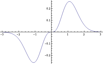
The integrand is an odd function (i.e. f(−x) = −f(x)), and the integrand of an odd function over a symmetric interval is zero. This is because the region below the x-axis is symmetric to the region above the x-axis as the following graph shows.

plot of x log(1 + x^2) exp(-x^2)

The example above is not artificial: similar calculations come up constantly in applications. For example, the Fourier series of an odd function contains only sine terms, no cosine terms. Why? The integrals to compute the Fourier coefficients for the cosine terms all involve odd functions integrated over an interval symmetric about zero.

Another common application of symmetry is evaluating derivatives. The derivative of an odd function is an even function and vice versa.

Pop quiz 2: What is the coefficient of x⁵ in the Taylor series of cos(1 + x²)?

Solution: Zero, by symmetry, because cos(1 + x²) is an even function.

Odd functions of x have only odd powers of x in their Taylor series and even functions have only even powers of x in their Taylor series. Why? Because the coefficients come from derivatives evaluated at zero.

If f(x) is an odd function, all of its even derivatives are odd functions. These derivatives are zero at x = 0, and so all the coefficients of even powers of x are zero. A similar argument shows that even functions have only even powers of x in their Taylor series.

Symmetry tricks are obvious in hindsight. The hard part is learning to recognize when they apply. Symmetries are harder to recognize, but also more valuable, in complex situations. The key is to think about the problem you’re trying to solve before you dive into heads-down calculation.

Three surprises with the trapezoid rule

Posted on 2 December 2010 by John

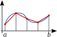
The trapezoid rule is a very simple method for estimating integrals. The idea is to approximate the area under a curve by a bunch of thin trapezoids and add up the areas of the trapezoids as suggested in the image below.

This is an old idea, probably older than the formal definition of an integral. In general it gives a crude estimation of the integral. If the width of the trapezoids is h, the error in using the trapezoid rule is roughly proportional to h². It’s easier to do better. For example, Simpson’s rule is a minor variation on the trapezoid rule that has error proportional to h⁵.

So if the trapezoid rule is old and inaccurate, why does anyone care about it? Here are the surprises.

You can still get a publication out of the trapezoid rule! In 1994, a doctor published a paper reinventing the trapezoid rule. Not only did the editors not recognize this ancient algorithm, the paper has been cited many times since it was published. (Update: more about the trapezoid paper here.)
Although the trapezoid rule is inefficient in general, it can be shockingly efficient for periodic functions.
The trapezoid rule can also be shockingly efficient for analytic functions that go to zero quickly, so called double exponential functions.

The last two observations are more widely applicable than you might think at first. What if you want to integrate something that isn’t periodic and isn’t a double exponential function? You may be able to do a change of variables that makes your integrand have one of these special forms. The article Fast Numerical Integration explains an integration method based on double exponential functions and includes C++ source code.

The potential efficiency of the trapezoid rule illustrates a general principle: a crude method cleverly applied can beat a clever technique crudely applied. The simplest numerical integration technique, one commonly taught in freshman calculus, can be extraordinarily efficient when applied with skill to the right problem. Conversely, a more sophisticated integration technique such as Gauss quadrature can fail miserably when naively applied.

Integration