Numerically integrating periodic functions

Posted on 1 March 2017 by John

The trapezoid rule is the most obvious numerical integration technique. It comes directly from the definition of a definite integral, just a Riemann sum.

It’s a very crude technique in general; you can get much more accuracy with the same number of function evaluations by using a more sophisticated method. But for smooth periodic functions, the trapezoid rule works astonishingly well.

This post will look at two similar functions. The trapezoid rule will be very accurate for one but not for the other. The first function is

g(x) = exp( cos(x) ).

The second function, h(x) replaces the cosine with its Taylor approximation 1 – x²/2. That is,

h(x) = exp(1 – x²/2 ).

The graph below shows both functions.

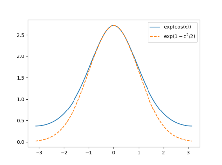
Both functions are perfectly smooth. The function g is naturally periodic with period 2π. The function h could be modified to be a periodic function with the same period since h(-π) = h(π).

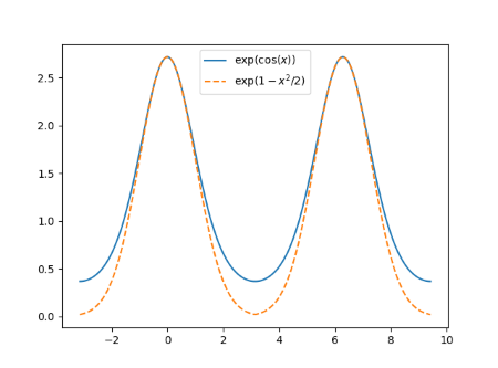
But the periodic extension of h is not smooth. It’s continuous, but it has a kink at odd multiples of π. The derivative is not continuous at these points. Here’s a close-up to show the kink.

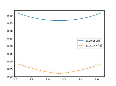
Now suppose we want to integrate both functions from -π to π. Over that range both functions are smooth. But the behavior of h “off stage” effects the efficiency of the trapezoid rule. Making h periodic by pasting copies together that don’t match up smoothly does not make it act like a smooth periodic function as far as integration is concerned.

Here’s the error in the numerical integration using 2, 3, 4, …, 10 integration points.

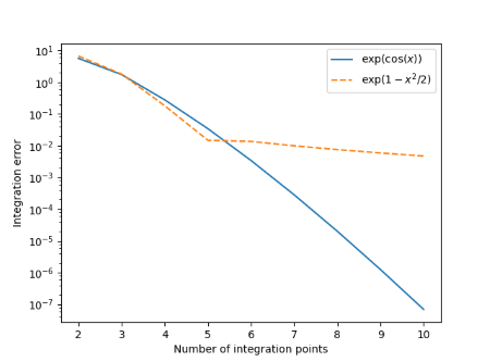
The integration error for both functions decreases rapidly as we go from 2 to 5 integration points. And in fact the integration error for h is slightly less than that for g with 5 integration points. But the convergence for h practically stops at that point compared to g where the integration error decreases exponentially. Using only 10 integration points, the error has dropped to approximately 7×10^-8 while the error for h is five orders of magnitude larger.

To read more along these lines, see J. A. C. Weideman’s article Numerical Integration of Periodic Functions: A Few Examples, The American Mathematical Monthly, Vol. 109, No. 1, pp. 21–36.

Simplify integration with complex variables

Posted on 24 January 2017 by John

Last night I was helping my daughter with her calculus homework. One of the problems was the following integral:

$\int \exp(-x) \sin(4x) \, dx$

This is an interesting problem for two reasons. First, it illustrates a clever variation on integration by parts; that’s why it was assigned. But it can also be computed using complex variables. As is often the case, the “complex” approach is simpler. Below I’ll show the solution the students were expected to find, then one that they wouldn’t not be expected to find.

Integration by parts

The traditional approach to this integral is to integrate by parts. Letting u = sin(4x), the integral becomes

$- \exp(-x) \sin(4x) + 4 \int \exp(-x) \cos(4x) \, dx$

Next we integrate by parts one more time, this time letting u = cos(4x). This gives us

$- \exp(-x) \sin(4x) - 4 \exp(-x) \cos(4x) -16\int \exp(-x) \sin(4x) \, dx$

At this point it looks like we’re getting nowhere. We could keep on integrating by parts forever. Not only that, we’re going in circles: we have an integral that’s just like the one we started with. But then the clever step is to realize that this is a good thing. Let I be our original integral. Then

$I = -\exp(x) \left(\sin(4x) + 4 \cos(4x)\right) - 16 I$

Now we can solve for I:

$I = - \frac{1}{17} \exp(-x) (\sin(4x) + 4 \cos(4x))$

Complex variables

Here’s another approach. Recognize that sin(4x) is the imaginary part of exp(4ix) and so our integral is the imaginary part of

$\int \exp(-x) \exp(-4ix) \,dx = \int \exp\left((-1+4i)x\right) \,dx$

which we can integrate immediately:

$\frac{1}{-1+4i} \exp\left((-1+4i)x\right).$

There’s still algebra to do, but the calculus is over. And while the algebra will take a few steps, it’s routine.

First, let’s take care of the fraction.

$\frac{1}{-1+4i} = \frac{1}{-1+4i} \frac{-1 - 4i}{-1 - 4i} = - \frac{1+4i}{17}.$

Next,

$\exp\left((-1+4i)x\right) = \exp(-x)\left( \cos(4x) + i \sin(4x) \right)$

and so our integral is the complex part of

$-\frac{1}{17} \exp(-x) (1 + 4i)\left( \cos(4x) + i \sin(4x) \right)$

which gives us the same result as before.

The complex variable requires one insight: recognizing a sine as the real part of an exponential. The traditional approach requires several insights: two integrations by parts and solving for the original integral.

An integral with a couple lessons

Posted on 7 December 2016 by John

If you present calculus students with a definite integral, their Pavlovian response is “Take the anti-derivative, evaluate it at the limits, and subtract.” They think that’s what it means. But it’s not what a definite integral means. It’s how you (usually) calculate its value. This is not a pedantic fine point but a practically important distinction. It pays to distinguish what something means from how you usually calculate it. Without this distinction, things that are possible may seem impossible. [1]

For example, suppose you want to compute the following integral that comes up frequently in probability.

$\int_{-\infty}^\infty e^{-x^2}\, dx$

There is no (elementary) function whose derivative is exp(-x²). It’s not just hard to find or ugly. It simply doesn’t exist, not within the universe of elementary functions. There are functions whose derivative is exp(-x²), but these functions are not finite algebraic combinations of the kinds of functions you’d see in high school.

If you think of the definite integral above as meaning “the result you get when you find an antiderivative, let its arguments go off to ∞ and -∞, and subtract the two limits” then you’ll never calculate it. And when you hear that the antiderivative doesn’t exist (in the world of functions you’re familiar with) then you might think that not only can you not calculate the integral, no one can.

In fact the integral is easy to calculate. It requires an ingenious trick [2], but once you see that trick it’s not hard.

Let I be the value of the integral. Changing the integration variable makes no difference, i.e.

$I = \int_{-\infty}^\infty e^{-x^2}\, dx = \int_{-\infty}^\infty e^{-y^2}\, dy$

and so

$I^2 = \left(\int_{-\infty}^\infty e^{-x^2}\, dx\right) \left( \int_{-\infty}^\infty e^{-y^2}\, dy\right) = \int_{-\infty}^\infty\!\int_{-\infty}^\infty e^{-x^2 - y^2} \, dx\, dy$

This integral can be converted to polar coordinates. Instead of describing the plane as an infinite square with x and y each going off to infinity in both directions, we can think of it as an infinite disk, with radius going off to infinity. The advantage of this approach is that the Jacobian of the change of variables gives us an extra factor of r that makes the exponential integral tractable.

$\int_0^{2\pi} \! \int_0^\infty e^{-r^2} r \, dr\, d\theta = \frac{1}{2} \int_0^{2\pi} 1\, d\theta = \pi$

From this we get I² = π and so I = √π.

This specific trick comes up occasionally. But more generally, it is often the case that definite integrals are easier to compute than indefinite integrals. One of the most common applications of complex analysis is computing such integrals through the magic of contour integration. This leads to a lesson closely related to the one above, namely that you may not have to do what it looks like you need to do. In this case, you don’t always need to compute indefinite integrals (anti-derivatives) as an intermediate step to compute definite integrals. [3]

Mathematics is filled with theorems that effectively say that you don’t actually have to compute what you conceptually need to compute. Sometimes you can get by with calculating much less.

* * *

[1] One frustration I’ve had working with statisticians is that many have forgotten the distinction between what they want to calculate and how they calculate it. This makes it difficult to suggest better ways of computing things.

[2] Lord Kelvin said of this trick “A mathematician is one to whom that is as obvious as that twice two makes four is to you. Liouville was a mathematician.”

[3] If you look back carefully, we had to compute the integral of exp(-r²) r, which you would do by first computing its anti-derivative. But we didn’t have to compute the anti-derivative of the original integrand. We traded a hard (in some sense impossible) anti-derivative problem for an easy one.

Yet another way to define fractional derivatives

Posted on 30 July 2016 by John

Fractional integrals are easier to define than fractional derivatives. And for sufficiently smooth functions, you can use the former to define the latter.

The Riemann-Liouville fractional integral starts from the observation that for positive integer n,

$I^n f(x) &\equiv& \int_a^{x} \int_a^{x_1} \cdots \int_a^{x_{n-1}} f(x_n)\,dx_n\, dx_{n-1} \cdots \,dx_1 \\ &=& \frac{1}{(n-1)!} \int_a^x (x-t)^{n-1} f(t)\, dt$

This motivates a definition of fractional integrals

$I^\alpha f(x) = \frac{1}{\Gamma(\alpha)} \int_a^x (x-t)^{\alpha-1} f(t)\, dt$

which is valid for any complex α with positive real part. Derivatives and integrals are inverses for integer degree, and we use this to define fractional derivatives: the derivative of degree n is the integral of degree –n. So if we could define fractional integrals for any degree, we could define a derivative of degree α to be an integral of degree -α.

Unfortunately we can’t do this directly since our definition only converges in the right half-plane. But for (ordinary) differentiable f, we can integrate the Riemann-Liouville definition of fractional integral by parts:

$I^\alpha f(x) = \frac{(x-a)^\alpha}{\Gamma(\alpha+1)} f(a) + I^{\alpha+1} f'(x)$

We can use the right side of this equation to define the left side when the real part of α is bigger than -1. And if f has two ordinary derivatives, we can repeat this process to define fractional integrals for α with real part bigger than -2. We can repeat this process to define the fractional integrals (and hence fractional derivatives) for any degree we like, provided the function has enough ordinary derivatives.

See previous posts for two other ways of defining fractional derivatives, via Fourier transforms and via the binomial theorem.

Introduction to MCMC

Posted on 23 January 2016 by John

Markov Chain Monte Carlo (MCMC) is a technique for getting your work done when Monte Carlo won’t work.

The problem is finding the expected value of f(X) where X is some random variable. If you can draw independent samples x_i from X, the solution is simple:

$E[ f(X) ] \approx \frac{1}{n} \sum_{i=1}^n f(x_i)$

When it’s possible to draw these independent samples, the sum above is well understood. It’s easy to estimate the error after n samples, or to turn it the other way around, estimate what size n you need so that the error is probably below a desired threshold.

MCMC is a way of making the approximation above work even though it’s not practical to draw independent random samples from X. In Bayesian statistics, X is the posterior distribution of your parameters and you want to find the expected value of some function of these parameters. The problem is that this posterior distribution is typically complicated, high-dimensional, and unique to your problem (unless you have a simple conjugate model). You don’t know how to draw independent samples from X, but there are standard ways to construct a Markov chain whose samples make the approximation above work. The samples are not independent but in the limit the set of samples has the same distribution as X.

MCMC is either simple or mysterious, depending on your perspective. It’s simple to write code that should work, eventually, in theory. Writing efficient code is another matter. And above all, knowing when your answer is good enough is tricky. If the samples were independent, the Central Limit Theorem would tell you how the sum should behave. But since the samples are dependent, all bets are off. Almost all we know is that the average on the right side converges to the expectation on the left side. Aside from toy problems there’s very little theory to tell you when your average is sufficiently close to what you want to compute.

Because there’s not much theory, there’s a lot of superstition and folklore. As with other areas, there’s some truth in MCMC superstition and folklore, but also some error and nonsense.

In some ways MCMC is truly marvelous. It’s disappointing that there isn’t more solid theory around convergence, but it lets you take a stab at problems that would be utterly intractable otherwise. In theory you can’t know when it’s time to stop, and in practice you can fool yourself into thinking you’ve seen convergence when you haven’t, such as when you have a bimodal distribution and you’ve only been sampling from one mode. But it’s also common in practice to have some confidence that a calculation has converged because the results are qualitatively correct: this value should be approximately this other value, this should be less than that, etc.

Bayesian statistics is older than Frequentist statistics, but it didn’t take off until statisticians discovered MCMC in the 1980s, after physicists discovered it in the 1950s. Before that time, people might dismiss Bayesian statistics as being interesting but impossible to compute. But thanks to Markov Chain Monte Carlo, and Moore’s law, many problems are numerically tractable that were not before.

Since MCMC gives a universal approach for solving certain kinds of problems, some people equate the algorithm with the problem. That is, they see MCMC as the solution rather than an algorithm to compute the solution. They forget what they were ultimately after. It’s sometimes possible to compute posterior probabilities more quickly and more accurately by other means, such as numerical integration.

High-dimensional integration

Posted on 19 July 2015 by John

Numerically integrating functions of many variables almost always requires Monte Carlo integration or some variation. Numerical analysis textbooks often emphasize one-dimensional integration and, almost as a footnote, say that you can use a product scheme to bootstrap one-dimensional methods to higher dimensions. True, but impractical.

Traditional numerical integration routines work well in low dimensions. (“Low” depends on context, but let’s say less than 10 dimensions.) When you have the choice of a well-understood, deterministic method, and it works well, by all means use it. I’ve seen people who are so used to problems requiring Monte Carlo methods that they use these methods on low-dimensional problems where they’re not the most efficient (or robust) alternative.

Monte Carlo

Except for very special integrands, high dimensional integration requires either Monte Carlo integration or some variation such as quasi-Monte Carlo methods.

As I wrote about here, naive Monte Carlo integration isn’t practical for high dimensions. It’s unlikely that any of your integration points will fall in the region of interest without some sort of importance sampler. Constructing a good importance sampler requires some understanding of your particular problem. (Sorry. No one-size-fits-all black-box methods are available.)

Quasi-Monte Carlo (QMC)

Quasi-Monte Carlo methods (QMC) are interesting because they rely on something like a random sequence, but “more random” in a sense, i.e. more effective at exploring a high-dimensional space. These methods work well when an integrand has low effective dimension. The effective dimension is low when nearly all the action takes place on a lower dimensional manifold. For example, a function may ostensibly depend on 10,000 variables, while for practical purposes 12 of these are by far the most important. There are some papers by Art Owen that say, roughly, that Quasi-Monte Carlo methods work well if and only if the effective dimension is much smaller than the nominal dimension. (QMC methods are especially popular in financial applications.)

While QMC methods can be more efficient than Monte Carlo methods, it’s hard to get bounds on the integration error with these methods. Hybrid approaches, such as randomized QMC can perform remarkably well and give theoretical error bounds.

Markov Chain Monte Carlo (MCMC)

Markov Chain Monte Carlo (MCMC) is a common variation on Monte Carlo integration that uses dependent random samples. In many applications, such as Bayesian statistics, you’d like to be able to create independent random samples from some probability distribution, but this is not practical. MCMC is a compromise. It produces a Markov chain of dependent samples, and asymptotically these samples have the desired distribution. The dependent nature of the samples makes it difficult to estimate error and to determine how well the integration estimates using the Markov chain have converged.

(Some people speak of the Markov chain itself converging. It doesn’t. The estimates using the Markov chain may converge. Speaking about the chain converging may just be using informal language, or it may betray a lack of understanding.)

There is little theory regarding the convergence of estimates from MCMC, aside from toy problems. An estimate can appear to have converged, while an important region of the integration problem remains unexplored. Despite its drawbacks, MCMC is the only game in town for many applications.

***

Numerical integration consulting

Integration by Darts

Posted on 1 April 2015 by John

dartboard

Monte Carlo integration has been called “Integration by Darts,” a clever pun on “integration by parts.” I ran across the phrase looking at some slides by Brian Hayes, but apparently it’s been around a while. The explanation that Monte Carlo is “integration by darts” is fine as a 0th order explanation, but it can be misleading.

Introductory courses explain Monte Carlo integration as follows.

Plot the function you want to integrate.
Draw a box that contains the graph.
Throw darts (random points) at the box.
Count the proportion of darts that land between the graph and the horizontal axis.
Estimate the area under the graph by multiplying the area of the box by the proportion above.

In principle this is correct, but this is far from how Monte Carlo integration is usually done in practice.

For one thing, Monte Carlo integration is seldom used to integrate functions of one variable. Instead, it is mostly used on functions of many variables, maybe hundreds or thousands of variables. This is because more efficient methods exist for low-dimensional integrals, but very high dimensional integrals can usually only be computed using Monte Carlo or some variation like quasi-Monte Carlo.

If you draw a box around your integrand, especially in high dimensions, it may be that nearly all your darts fall outside the region you’re interested in. For example, suppose you throw a billion darts and none land inside the volume determined by your integration problem. Then the point estimate for your integral is 0. Assuming the true value of the integral is positive, the relative error in your estimate is 100%. You’ll need a lot more than a billion darts to get an accurate estimate. But is this example realistic? Absolutely. Nearly all the volume of a high-dimensional cube is in the “corners” and so putting a box around your integrand is naive. (I’ll elaborate on this below. [1])

So how do you implement Monte Carlo integration in practice? The next step up in sophistication is to use “importance sampling.” [2] Conceptually you’re still throwing darts at a box, but not with a uniform distribution. You find a probability distribution that approximately matches your integrand, and throw darts according to that distribution. The better the fit, the more efficient the importance sampler. You could think of naive importance sampling as using a uniform distribution as the importance sampler. It’s usually not hard to find an importance sampler much better than that. The importance sampler is so named because it concentrates more samples in the important regions.

Importance sampling isn’t the last word in Monte Carlo integration, but it’s a huge improvement over naive Monte Carlo.

***

[1] So what does it mean to say most of the volume of a high-dimensional cube is in the corners? Suppose you have an n-dimensional cube that runs from -1 to 1 in each dimension and you have a ball of radius 1 inside the cube. To make the example a little simpler, assume n is even, n = 2k. Then the volume of the cube is 4^k and the volume of the sphere is π^k / k!. If k = 1 (n = 2) then the sphere (circle in this case) takes up π/4 of the volume (area), about 79%. But when k = 100 (n = 200), the ball takes up 3.46×10^-169 of the volume of the cube. You could never generate enough random samples from the cube to ever hope to land a single point inside the ball.

[2] In a nutshell, importance sampling replaces the problem of integrating f(x) with that of integrating (f(x) / g(x)) g(x) where g(x) is the importance sampler, a probability density. Then the integral of (f(x) / g(x)) g(x) is the expected value of (f(X) / g(X)) where X is a random variable with density given by the importance sampler. It’s often a good idea to use an importance sampler with slightly heavier tails than the original integrand.

Integration trick

Posted on 22 October 2014 by John

Here’s a clever example from Paul Nahin’s new book Inside Interesting Integrals. Suppose you want to evaluate

$\int_{-1}^1 \frac{\cos(x)}{\exp(1/x) + 1}\,dx$

Since the range of integration is symmetric around zero, you might think to see whether the integrand is an odd function, in which case the integral would be zero. (More on such symmetry tricks here.) Unfortunately, the integrand is not odd, so that trick doesn’t work directly. However, it does help indirectly.

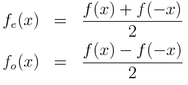
You can split any function f(x) into its even and odd parts.

$f_e(x) = \frac{f(x) + f(-x)}{2} \\ f_o(x) = \frac{f(x) - f(-x)}{2}$

The integral of a function over a symmetric interval is the integral of its even part because its odd part integrates to zero. The even part of the integrand above works out to be simply cos(x)/2 and so the integral evaluates to sin(1).

How Lp spaces nest

Posted on 11 November 2012 by John

A function f(x) is said to be in L^p if the integral of |f(x)|^p is finite. So if you know f is in L^p for some value of p, can conclude that f is also in L^q for some q? In general, no. But for two important special cases, yes. The special cases have to do with the domain of f.

If f is a function on a finite measure space and p > q, then every function in L^p is in L^q. In particular probability spaces are finite measure spaces, and so if a random variable’s pth moment exists, the qth moment exists.

If the domain of f is the integers with counting measure, f is a sequence and the “integral” of |f(x)|^p is simply a sum. Now the relationship between L^p spaces is reversed: p > q, every sequence in L^q is in L^p.

There are two reasons a function could fail to be in L^p: singularities and fat tails. In a finite measure space, there are no tails; you only have to worry about singularities. On the integers, there are no singularities; you only have to worry about tails.

Now consider functions on the whole real line. Membership in L^p says nothing about membership in L^q because now you can have singularities and fat tails.

Avoiding underflow in Bayesian computations

Posted on 26 July 2012 by John

Here’s a common problem that arises in Bayesian computation. Everything works just fine until you have more data than you’ve seen before. Then suddenly you start getting infinite, NaN, or otherwise strange results. This post explains what might be wrong and how to fix it.

A posterior density is (proportional to) a likelihood function times a prior distribution. The likelihood function is a product. The number of data points is the number of terms in the product. If these numbers are less than 1, and you multiply enough of them together, the result will be too small to represent in a floating point number and your calculation will underflow to zero. Then subsequent operations with this number, such as dividing it by another number that has also underflowed to zero, may produce an infinite or NaN result.

The instinctive reaction regarding underflow or overflow is to use logs. And often that works. If you wanted to know where the maximum of the posterior density occurs, you could find the maximum of the logarithm of the posterior density. But in Bayesian computations you often need to integrate the posterior density times some functions. Now you cannot just work with logs because logs and integrals don’t commute.

One way around the problem is to multiply the integrand by a constant so large that there is no danger of underflow. Multiplying by constants does commute with integration.

So suppose your integrand is on the order of 10^-400, far below the smallest representable number. Do you need extended precision arithmetic? No, you just need to understand your problem.

If you multiply your integrand by 10^400 before integrating, then your integrand is roughly 1 in magnitude. Then do you integration, and remember that the result is 10^400 times the actual value.

You could take the following steps.

Find m, the maximum of the log of the integrand.
Let I be the integral of exp( log of the integrand – m ).
Keep track that your actual integral is exp(m) I, or that its log is m + log I.

Note that you can be extremely sloppy in this process. You don’t need an accurate estimate of the maximum of the integrand per se. If you’re within a few dozen orders of magnitude, for example, that could be sufficient to carry out your integration without underflow.

One way to estimate the maximum is to use a frequentist estimator of your parameters as an approximate MLE, and assume that this is approximately where your posterior density takes on its maximum value. This might actually be very accurate, but it doesn’t need to be.

Note also that it’s OK if some of the evaluations of your integrand underflow to zero. You just don’t want the entire integral to underflow to zero. Places where the integrand is many orders of magnitude less than its maximum don’t contribute to the integration anyway. (It’s important that your integration pays attention to the region where the integrand is largest. A naive integration could entirely miss the most important region and completely underestimate the integral. But that’s a matter for another blog post.)

Integration by parts

Complex variables

Related posts

Monte Carlo

Quasi-Monte Carlo (QMC)

Markov Chain Monte Carlo (MCMC)