I’ve written a couple posts lately on getting an LLM to generate code to solve chess problems. The first used Claude to generate Prolog and the second used ChatGPT to generate Prolog. This post will use Claude to generate Z3/Python code.

The puzzle is one I’ve written about before:

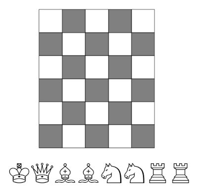
Place all the pieces—king, queen, two bishops, two knights, and two rooks—on a 6 × 5 chessboard, with the requirement that the two bishops be on opposite colored squares and no piece is attacking another.

Incidentally, it’s common for “piece” to exclude pawns, as above. But then what do you call all the things on a chessboard? You might call them “chess pieces,” in which case a pawn is a “chess piece” but not a “piece.” One convention is to use “chessmen” or simply “men” to include pieces and pawns.

This was the prompt I used.

Write Z3/Python code to find all solutions to the following chess puzzle.

Place all the pieces—king, queen, two bishops, two knights, and two rooks—on a 6 × 5 chessboard, with the requirement that the two bishops be on opposite colored squares and no piece is attacking another.

The code found 192 = 8 × 24 solutions. The factor of 8 comes from 2³ ways of swapping the pairs of bishops, knights, and rooks. The script reports

Total raw solutions: 192
Unique solutions (deduplicating piece-pair swaps): 24

── Solution 1 ──
  0 1 2 3 4
0 . K . . N
1 . . . . B
2 . . R . .
3 Q . . . .
4 . . . R .
5 . B . . N
  King: (0,1)
  Queen: (3,0)
  Bishop1: (5,1) [light]
  Bishop2: (1,4) [dark]
  Knight1: (5,4)
  Knight2: (0,4)
  Rook1: (4,3)
  Rook2: (2,2)

── Solution 2 ──
  0 1 2 3 4
0 N . . K .
1 B . . . .
2 . . R . .
3 . . . . Q
4 . R . . .
5 N . . B .
  King: (0,3)
  Queen: (3,4)
  Bishop1: (5,3) [light]
  Bishop2: (1,0) [dark]
  Knight1: (5,0)
  Knight2: (0,0)
  Rook1: (4,1)
  Rook2: (2,2)

...

── Solution 24 ──
  0 1 2 3 4
0 B . . B .
1 N . . . .
2 . . . . Q
3 . . R . .
4 . R . . .
5 N . . K .
  King: (5,3)
  Queen: (2,4)
  Bishop1: (0,0) [light]
  Bishop2: (0,3) [dark]
  Knight1: (5,0)
  Knight2: (1,0)
  Rook1: (3,2)
  Rook2: (4,1)

Here’s the code.

"""
Chess Puzzle Solver using Z3
Place king, queen, 2 bishops, 2 knights, 2 rooks on a 6×5 board
such that:
  - The two bishops are on opposite-colored squares
  - No piece attacks any other piece
"""

from z3 import (
    Int, Solver, Or, And, Not, Distinct, If,
    sat, ForAll, Implies
)
import itertools

ROWS = 6
COLS = 5
TOTAL_CELLS = ROWS * COLS  # 30

PIECES = ["king", "queen", "bishop1", "bishop2", "knight1", "knight2", "rook1", "rook2"]
N = len(PIECES)  # 8 pieces

def cell(r, c):
    return r * COLS + c

def pos_to_rc(pos):
    return pos // COLS, pos % COLS

def color(r, c):
    """Square color: 0=light, 1=dark"""
    return (r + c) % 2

def attacks_king(r1, c1, r2, c2):
    return max(abs(r1 - r2), abs(c1 - c2)) == 1

def attacks_queen(r1, c1, r2, c2):
    return (r1 == r2 or c1 == c2 or
            abs(r1 - r2) == abs(c1 - c2))

def attacks_bishop(r1, c1, r2, c2):
    return abs(r1 - r2) == abs(c1 - c2)

def attacks_rook(r1, c1, r2, c2):
    return r1 == r2 or c1 == c2

def attacks_knight(r1, c1, r2, c2):
    dr, dc = abs(r1 - r2), abs(c1 - c2)
    return (dr == 1 and dc == 2) or (dr == 2 and dc == 1)

# Map piece index to its attack function
ATTACK_FN = {
    0: attacks_king,
    1: attacks_queen,
    2: attacks_bishop,
    3: attacks_bishop,
    4: attacks_knight,
    5: attacks_knight,
    6: attacks_rook,
    7: attacks_rook,
}

def solve_all():
    solutions = []

    # Each piece gets an integer position in [0, TOTAL_CELLS)
    pos = [Int(f"pos_{p}") for p in PIECES]

    s = Solver()

    # All positions in valid range
    for p in pos:
        s.add(p >= 0, p < TOTAL_CELLS)

    # All pieces on distinct squares
    s.add(Distinct(*pos))

    # Bishops on opposite colors
    # bishop1 = pos[2], bishop2 = pos[3]
    # color of pos = ((pos // COLS) + (pos % COLS)) % 2
    b1_color = (pos[2] / COLS + pos[2] % COLS) % 2  # Z3 integer arithmetic
    b2_color = (pos[3] / COLS + pos[3] % COLS) % 2

    # Z3 doesn't do Python //; use integer division carefully
    # We'll encode opposite colors: sum of colors == 1
    # color(pos) = (row + col) % 2 = (pos//COLS + pos%COLS) % 2
    # For Z3 int vars, use: (pos / COLS + pos % COLS) % 2
    s.add((pos[2] / COLS + pos[2] % COLS) % 2 != (pos[3] / COLS + pos[3] % COLS) % 2)

    # No piece attacks another
    # We enumerate all (i,j) pairs and for each possible (pos_i, pos_j) assignment,
    # assert that those pieces don't attack each other.
    # Since positions are Z3 vars, we use a constraint table approach:
    # For each pair (i,j), add constraints over all concrete (r1,c1,r2,c2) combos.

    # Pre-build attack lookup tables for each piece-type pair
    # This avoids slow Z3 symbolic reasoning over large disjunctions.

    # We'll encode: for all concrete assignments, if pos[i]==cell(r1,c1) and pos[j]==cell(r2,c2),
    # then piece i must not attack piece j.
    # Equivalently: NOT (pos[i]==cell(r1,c1) AND pos[j]==cell(r2,c2)) for all attacking pairs.

    # For efficiency, we build a set of "forbidden (cell_i, cell_j)" pairs per piece pair.

    for i, j in itertools.combinations(range(N), 2):
        fn_i = ATTACK_FN[i]
        fn_j = ATTACK_FN[j]
        forbidden = []
        for r1, c1 in itertools.product(range(ROWS), range(COLS)):
            for r2, c2 in itertools.product(range(ROWS), range(COLS)):
                if (r1, c1) == (r2, c2):
                    continue
                # i attacks j or j attacks i
                if fn_i(r1, c1, r2, c2) or fn_j(r2, c2, r1, c1):
                    forbidden.append((cell(r1, c1), cell(r2, c2)))

        if forbidden:
            # Add: NOT (pos[i] == ci AND pos[j] == cj) for each forbidden pair
            s.add(And([
                Not(And(pos[i] == ci, pos[j] == cj))
                for ci, cj in forbidden
            ]))

    # Enumerate all solutions
    solution_count = 0
    while s.check() == sat:
        m = s.model()
        sol = [m[pos[k]].as_long() for k in range(N)]
        solutions.append(sol)
        solution_count += 1

        # Block this solution (and symmetric duplicates via blocking exact assignment)
        s.add(Or([pos[k] != sol[k] for k in range(N)]))

        if solution_count % 10 == 0:
            print(f"  Found {solution_count} solutions so far...")

    return solutions

def print_board(sol):
    board = [["." for _ in range(COLS)] for _ in range(ROWS)]
    symbols = ["K", "Q", "B", "B", "N", "N", "R", "R"]
    for k, p in enumerate(sol):
        r, c = pos_to_rc(p)
        board[r][c] = symbols[k]
    print("  " + " ".join(str(c) for c in range(COLS)))
    for r in range(ROWS):
        print(f"{r} " + " ".join(board[r]))

def canonicalize(sol):
    """
    Produce a canonical form to deduplicate solutions where
    bishop1/bishop2, knight1/knight2, rook1/rook2 are interchangeable.
    Returns a frozenset-based key.
    """
    king_pos   = sol[0]
    queen_pos  = sol[1]
    bishops    = tuple(sorted([sol[2], sol[3]]))
    knights    = tuple(sorted([sol[4], sol[5]]))
    rooks      = tuple(sorted([sol[6], sol[7]]))
    return (king_pos, queen_pos, bishops, knights, rooks)

def main():
    print("Solving chess puzzle on 6×5 board...")
    print("Pieces: King, Queen, 2 Bishops (opposite colors), 2 Knights, 2 Rooks")
    print("Constraint: No piece attacks another\n")

    solutions = solve_all()

    # Deduplicate by canonical form
    seen = {}
    for sol in solutions:
        key = canonicalize(sol)
        if key not in seen:
            seen[key] = sol

    unique = list(seen.values())
    print(f"\nTotal raw solutions: {len(solutions)}")
    print(f"Unique solutions (deduplicating piece-pair swaps): {len(unique)}\n")

    for idx, sol in enumerate(unique, 1):
        print(f"── Solution {idx} ──")
        print_board(sol)
        labels = ["King", "Queen", "Bishop1", "Bishop2", "Knight1", "Knight2", "Rook1", "Rook2"]
        for k, p in enumerate(sol):
            r, c = pos_to_rc(p)
            col_name = "light" if color(r, c) == 0 else "dark"
            sq = f"({r},{c})"
            extra = f" [{col_name}]" if "Bishop" in labels[k] else ""
            print(f"  {labels[k]}: {sq}{extra}")
        print()

if __name__ == "__main__":
    main()

Related post: Lessons Learned With the Z3 SAT/SMT Solver