The previous post pointed out the analogy between models for modal logic (i.e. Kripke semantics) and science fiction. Rules for relationships between points in a Kripke model are analogous to rules for interplanetary travel in a fictional universe. This post will expand on this last point.
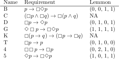
The following cube shows the relationships between eight different axiom systems for modal logic. Unfortunately, as I’ve written about before, the names of these systems are more historical than mnemonic.
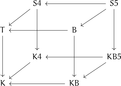
An arrow from A to B means the set of propositions provable in A contain the propositions provable in B.
For example, all the systems represent by the cube are “normal,” meaning that they all require Axiom K. So any proposition provable in K is provable in the other systems as well.
The axes of the cube correspond to rules for how “worlds” are connected in Kripke models. Imagine that K in the diagram is the origin. The x axis (from K to KB) corresponds to symmetry, the y axis (from K to K4) corresponds to transitivity, and the z axis (from K to T) corresponds to reflexivity.
S4 example
S4 in the diagram has coordinates (0, 1, 1), meaning that Kripke models for S4 must be transitive and reflexive. In SF terms, this says you can travel from any planet back to itself, and if it is possible to travel from planet x to planet y, and possible to travel from planet y to planet z, then it must be possible to travel from x to y.
Why weaker systems than S5?
Models of S5 are symmetric: if you can travel from x to y, you can travel from y to x. S4 does not have this requirement.
The axioms for S5 seem so sensible that you may wonder what the point is in having weaker systems. It all depends on how you interpret the modal qualifier □. In some applications of modal logic, □ has properties that correspond to models with unusual restrictions on accessibility.
We’re not trying to use logic to describe networks, though we could, but rather creating networks to model systems of logic. The resulting networks may have strange geometry if they weren’t motivated by geometry to begin with.
Axiom K
Axiom K (named for Saul Kripke) requires that
□(p → q) → (□p → □q)
This says that if the proposition p → q is true in all accessible worlds, and if p is true in all accessible worlds, then q must be true in all accessible worlds.
Axiom T
Axiom T requires that
□p →p.
If something is true in all worlds accessible from a world w, and w is accessible from itself, then it must be true on w.
Axiom 4
Axiom 4 requires
□p → □□p.
Standing on a world w, the proposition □p says that p is true on all worlds accessible from w. So if x is a world accessible from w, p is true there. And if y is a world accessible from x, then by transitivity that world must be accessible from x, so p is true there. So □p is true on x. And since □p is true on any world accessible from w, then we can say □□p.
Axiom B
Axiom B requires
p → □◇p.
One way to state this is that if a proposition is true, then it is necessarily possibly true.
Imagine you’re on a world w there p is true. Symmetry says that if a world x accessible from w, then w is accessible from x. Now □◇p holds because in any world x accessible from w, we have ◇p because w is accessible from x.
Axiom 5
Axiom 5 requires
◇p →□◇p.
In words, whatever is possible is necessarily possible. A Kripke model for axiom 5 must be Euclidean: If from world w you can access worlds x and y, then from x you can access y. A relation that is symmetric and transitive is Euclidean. If x is accessible from w, then symmetry says w is accessible from x, and transitivity says you can go on from w to y.
Systems versus Axioms
One of the confusing things about modal logic is the complicated relation between the names of axioms and systems of axioms. Sometimes it’s simple. For example, K4 means the system with axioms K and 4.
The vertices of the cube above are systems, not axioms. And system B, confusingly, requires more than axiom B, and is in fact stronger than system KB because it adds axiom T. Chellas [1] calls this system KTB, a more verbose but more transparent name.
Provenance of the cube
The cube at the top of this post is a simplification of similar diagrams that appear in The Standford Encyclopedia of Philosophy and Wikipedia. Both may trace their origin to figure 4.1 in [1]. I don’t know that either diagram came from there, or whether they were developed independently, but [1] predates both. However, the graph in Chellas is less clear. The edge directions are implicit, as is the connection to properties of the models.
Related posts
[1] Brian F. Chellas. Modal Logic: An Introduction. 1980,
![\begin{table}[] \begin{tabular}{lccll} & \phantom{i}add\phantom{i} & mult & & \\ \cline{2-3} \multicolumn{1}{l|}{conjunction} & \multicolumn{1}{c|}{\&} & \multicolumn{1}{c|}{\otimes} & & \\ \cline{2-3} \multicolumn{1}{r|}{disjunction} & \multicolumn{1}{c|}{\oplus} & \multicolumn{1}{c|}{\parr} & & \\ \cline{2-3} & & & & \end{tabular} \end{table}](https://www.johndcook.com/linear_con_dis_add_mult.png)
![\begin{table}[] \begin{tabular}{lcccl} & add & mult & exp & \\ \cline{2-4} \multicolumn{1}{r|}{positive} & \multicolumn{1}{c|}{\oplus} & \multicolumn{1}{c|}{\otimes} & \multicolumn{1}{c|}{!} & \\ \cline{2-4} \multicolumn{1}{r|}{negative} & \multicolumn{1}{c|}{\&} & \multicolumn{1}{c|}{\parr} & \multicolumn{1}{c|}{?} & \\ \cline{2-4} \end{tabular} \end{table}](https://www.johndcook.com/linear_pos_neg_add_mult_exp.png)
![data = [0, 0, 0, 0, 4, 44, 145, 339, 296, 128, 38, 5, 0, 1]](https://www.johndcook.com/bool_hist.png)

