DNA Sequence Alignment and Kings

Posted on 30 June 2026 by John

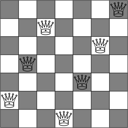
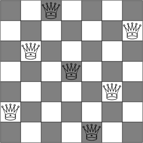
This morning I wrote a post that included the central Delannoy numbers. The nth central Delannoy number D_n counts the number of ways a king can move from one corner of a chessboard to the diagonally opposite corner without backtracking.

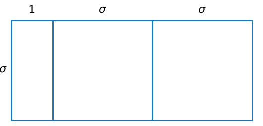
The more general Delannoy numbers D_m,n are the analogy for an m × n rectangular board, not necessarily square.

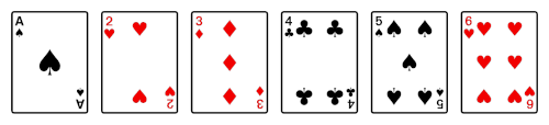
D_m,n is also the number of possible sequence alignments for a strand of DNA with m base pairs and a strand with n base pairs [1]. At each step in the alignment process, you can introduce a gap in the first strand, the second strand or neither, which is analogous to the king who can move N, E, or NE at each step.

The Delannoy numbers can be computed recursively:

def D(m, n):
    if m == 0 or n == 0:
        return 1
    return D(m - 1, n) + D(m, n - 1) + D(m - 1, n - 1)

The code above can be sped up tremendously by adding the decorator

@lru_cache(maxsize=None)

above the function definition to turn on memoization. I did an experiment computing D_12,15 with and without memoization and the times were 77.1805 seconds and 0.000062 seconds respectively, i.e. memoization made the code over a million times faster.

Incidentally, D_12,15 = 2653649025 and so there are a lot of ways to align even short sequences unless you place some restriction on the permissible alignments.

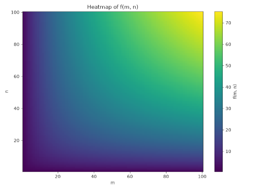
Update: Here’s a heatmap plotting log₁₀(D_m,n). Obviously the function increases with m and n: bigger chessboards have more possible paths. Moreover, it’s larger along the diagonal (i.e. the central Delannoy numbers). If you look along northeast to southwest diagonals, the function is largest in the middle where m = n.

[1] Torres, A., Cabada, A., & Nieto, J. J. (2003). An exact formula for the number of alignments between two DNA sequences. DNA Sequence, 14(6), 427–430. https://doi.org/10.1080/10425170310001617894

Silver Rectangles and the Ways of Kings

Posted on 30 June 2026 by John

Golden rectangles

The defining property of golden rectangle is that if you stick a square on its longer side, you get another golden rectangle.

The smaller vertical rectangle is similar to the larger horizontal rectangle. This means

φ / 1 = (1 + φ) / φ

which tells us φ² = 1 + φ and so the golden ratio φ equals (1 + √5)/2.

Silver rectangles

A silver rectangle is one that if you stick two squares on its longer side you get another rectangle with the same aspect ratio.

This tells us

σ / 1 = (1 + 2σ) / σ

and so σ² = 1 + 2σ and the silver ratio is σ = 1 + √2.

Just as you can define a golden ratio and a silver ratio, there’s an analogous way to define a sequence of metallic ratios.

Kings and Delannoy numbers

The silver ratio has several connections to the ways of ways kings. By that I mean the number of ways a king can go from one corner of a chessboard to the diagonally opposite corner without backtracking.

A king can move one space in any direction. If we start with a king in the bottom left corner of the board, the no-backtracking requirement means the king can move up, right, or up and right.

The number of paths a king can take from one corner to the opposite corner of an n × n chessboard is the nth central Delannoy number D_n. more generally Delannoy numbers are defined for an m × n chessboard, but I’ll stick to the case m = n called the central Delannoy number, or just Delannoy numbers for short.

The first Delannoy number is 1 because there’s only one way for a king to get from one corner to the other: do nothing, because the opposite corner is the same corner. The second Delannoy number is 3 because the king can move up then right, or right then up, or move diagonally up and right.

For a 3 × 3 grid things are significantly more complicated, and D₃ = 13. For an 8 × 8 grid the number of paths is 48,639.

Generating function

How would you estimate the number of paths on an n × n board for large values of n without calculating it exactly? You might start by finding a generating function for the Delannoy numbers, which works out to be

(x² − 6x + 1)^−1/2

The radius of convergence r for the generating function series is the distance from 0 to the closest singularity of the generating function, which is the smaller root of

x² − 6x + 1

which is

3 − √8 = (3 + √8)⁻¹ = (1 + √2)⁻² = 1/σ²

i.e. the radius of convergence is the reciprocal of the silver ratio squared.

Asymptotic estimate

The radius of convergence gives us a first approximation to the asymptotic size of the series coefficients. Since we’re working with the generating function of the Delannoy numbers, these coefficients are the Delannoy numbers. That is,

D_n ~ r⁻ⁿ = (σ²)ⁿ = σ²ⁿ.

That’s as good as you can do just knowing the radius of convergence. A more careful analysis would refine this estimate by dividing by a factor proportional to √n.

Queens on a prime order board

Posted on 21 June 2026 by John

The n queens problem is to place on an n × n chessboard n queens so that none attacks any other. This means there is only one queen on every horizontal, vertical, and diagonal line.

When n is a prime number ≥ 5, it is sufficient to place the queens on a line that has slope 2, 3, 4, …, n − 2. (The slope cannot be 1 because that’s a diagonal. And it cannot be n − 1 because n − 1 = −1 mod n is also a diagonal.) [1]

Here we imagine opposite edges of the board being joined together. Geometrically, this makes the chessboard a torus (donut). Algebraically, the points on a line of slope s have the coordinates

(a + k, b + ks)

where addition is carried out mod n.

All solutions to the n queens problem have this form when n = 5. Some solutions will have this form for larger prime values of n but not all.

For example, when n = 7, here is a solution where all the queens are on a line of slope 2.

But here is another solution where the queens do not all lie on a line of constant slope.

[1] W. H. Bussey. A Note on the Problem of the Eight Queens. The American Mathematical Monthly, Vol. 29, No. 7 (August 1922), pp. 252–253

Partitions over permutations

Posted on 4 June 2026 by John

I was thinking more about the cosine approximation to the Gaussian

exp(−z²) ≈ (1 + cos(sin(z) + z))/2

that I wrote about last week. The two expressions above are close along the real axis but not along the imaginary axis.

If z = iy, the right side grows much faster than the left, behaving like exp(exp(y)).

This led to me looking up the power series for the double exponential function exp(exp(y)). This is an interesting series because the coefficient of xⁿ is

e B_n / n!

where B_n is the nth Bell number, which equals the number of ways to partition a set of n labeled items [1]. And of course n! is the number of ways to permute a set of n labeled items. So the nth coefficient in the power series for exp(exp(y)) is the ratio of the number of partitions to permutations for a set of n labeled things, multiplied by e.

The number of ways to partition a set of n things grows quickly as n increases, almost as quickly as the number of permutations, and so the series for the double exponential function converges very slowly.

Computing

SymPy has a function bell for computing Bell numbers, so you could compute the ratio of partitions to permutations as follows.

from sympy import bell, factorial
f = lambda n: bell(n)/factorial(n)

This returns a number of type sympy.core.numbers.Rational and so the result is exact. You can cast it to float for convenience.

Asymptotics

If we look at only the terms in the asymptotic series for log B_n and log n! that grow with n we have

log B_n ~ n log n − n log log n
log n! ~ n log n − ½ log n

and so

log( B_n / n! ) ~ ½ log n − n log log n

There’s also an asymptotic series for log( B_n / n! ) involving the Lambert W function:

log( B_n / n! ) ~ n/r − 1 − n log r

where r = W(n).

[1] It’s important that the items are labeled. Partition numbers are the number of partitions of an unlabeled set. Partition numbers are much smaller than Bell numbers.

Tone row operations

Posted on 17 March 2026 by John

The previous post introduced the idea of a twelve-tone row, a permutation of the twelve pitch classes of a chromatic scale.

The earlier post also introduced a group of operations on a tone row with elements P, R, I, and RI. Here P, which stands for “prime”, is the identity operator: it leaves the tone row alone. R stands for retrograde, which means to reverse the sequence. I stands for inversion, inverting each of the intervals in the row. If you apply R then I, you get the same result as if you first applied I then R. See the previous post for an example of each.

Do these operations always return a new tone row? In other words, are P(t), R(t), I(t), and RI(t) always distinct for all tone rows t?

It’s easy to see that P(t) and R(t) are always different. The first and last elements of t are different, and so the first element of P(t) does not equal the first element of R(t).

There is one interval that remains the same when inverted, namely the tritone. It’s possible to create a two-tone row that does not change under inversion, such as the sequence [B, F]. A tone row with more than two notes must have an interval that is not a tritone, and so inverting the tone row changes it.

If a tone row t has at least three notes, then P(t), R(t), I(t), and RI(t) are all distinct.

The pitch classes in a tone row are repeated in a cycle, so we might consider all rotations of a tone row to be in a sense the same. In mathematical terms, we can mod out by cyclic permutations.

If we apply R, I, and RI to equivalence classes of tone rows, the results are not always unique. For example, let t be the chromatic scale.

C C♯ D D♯ E F F♯ G G♯ A A♯ B

Then R(t) is

B A♯ A G♯ G F♯ F E D♯ D C♯ C

and I(t) is

C B A♯ A G♯ G F♯ F E D♯ D C♯

which is a rotation of R(t).

The chromatic scale is a boring tone row. For a random tone row t, all the variations P(t), R(t), I(t), and RI(t) will very likely be distinct, including rotations. The following Python code will illustrate the points above and estimate the probability that manipulations of a tone row are distinct even when equating rotations.

import random
import itertools

def inversion(x, m = 12):
    return [(2*x[0] - x[i]) % m for i in range(m)]

def rotate_left(x, n):
    return x[n:] + x[:n]

def rotdiff(x, y):
    for i in range(len(x)):
        if rotate_left(x, i) == y:
            return False
    return True

c = 0
for _ in range(1_000_000):
    P = list(range(12))
    random.shuffle(P) # shuffle in place
    R = list(reversed(P))
    I = list(inversion(P))
    RI = list(reversed(I))
    for pair in combinations([P, R, I, RI], 2):
        assert(pair[0] != pair[1])
        if not rotdiff(pair[0], pair[1]):
            c += 1
print(c)

This generates and tests a million random tone rows. When I ran it, it found 226 tone rows were one manipulation of the tone row was equal to a rotation of another. So when I said the variations are “very likely” to be distinct, you could quantify that as having over a 99.9% chance.

Combining in-shuffles and out-shuffles

Posted on 12 January 2026 by John

A few days ago I wrote two posts about perfect shuffles. Once you’ve cut a deck of cards in half, an in-shuffle lets a card from the top half fall first, and an out-shuffle lets a card from the bottom half fall first.

Suppose we have a deck of 52 cards. We said in the earlier posts that the order of an in-shuffle I is 52. That is, after 52 in-shuffles, a deck returns to its initial order. And the order of an out-shuffle O is 8.

We can think of I and O as generators of subgroups of order 52 and 8 respectively in the group S of all permutations of 52 cards. I was curious when I wrote the earlier posts how large the group generated by I and O together would be. Is it possible to reach all 52! permutations of the deck by some combination of applying I and O? If not, how many permutations can be generated?

I’ve since found the answer in [1] in a theorem by Diaconis, Graham, and Kantor. I don’t know who Kantor is, but it’s no surprise that a theorem on card shuffles would come from Persi Diaconis and Ron Graham. The theorem covers the case for decks of size N = 2n, which branches into different results depending on the size of n and the value of n mod 4.

For N = 52, the group generated by I and O has

26! × 2²⁶

elements.

On the one hand, that’s a big number, approximately 2.7 × 10³⁴. On the other hand, it’s quite small compared to 52! = 8 × 10⁶⁷. So while there are a lot of permutations reachable by a combination of in-shuffles and out-shuffles, your chances of selecting such a permutation from the set of all such permutations is vanishingly small.

To put it yet another way, the number of arrangements is on the order of the square root of 52!, a big number, but not big relative to 52!. (Does this pattern

√52! ≈ 26! × 2²⁶

generalize? See the next post.)

Not only does the theorem of Diaconis et al give the order of the group, it gives the group itself: the group of permutations generated by I and O is isomorphic to the group of symmetries of a 26-dimensional octahedron.

[1] S. Brent Morris. Magic Tricks, Card Shuffling and Dynamic Computer Memories. MAA 1998.

In-shuffles and out-shuffles

Posted on 1 January 2026 by John

The previous post talked about doing perfect shuffles: divide a deck in half, and alternately let one card from each half fall.

It matters which half lets a card fall first. If the top half’s bottom card falls first, this is called an in-shuffle. If the bottom half’s bottom card falls first, it’s called an out-shuffle.

With an out-shuffle, the top and bottom cards don’t move. Presumably it’s called an out-shuffle because the outside cards remain in place.

An out-shuffle amounts to an in-shuffle of the inner cards, i.e. the rest of the deck not including the top and bottom card.

The previous post had a Python function for doing an in-shuffle. Here we generalize the function to do either an in-shuffle or an out-shuffle. We also get rid of the list comprehension, making the code longer but easier to understand.

def shuffle2(deck, inside = True):
    n = len(deck)
    top = deck[: n//2]
    bottom = deck[n//2 :]
    if inside:
        first, second = bottom, top
    else:
        first, second = top, bottom
    newdeck = []
    for p in zip(first, second):
        newdeck.extend(p)
    return newdeck

Let’s use this code to demonstrate that an out-shuffle amounts to an in-shuffle of the inner cards.

deck = list(range(10))
d1 = shuffle2(deck, False) 
d2 = [deck[0]] + shuffle2(deck[1:9], True) + [deck[9]]
print(d1)
print(d2)

Both print statements produce [0, 5, 1, 6, 2, 7, 3, 8, 4, 9].

I said in the previous post that k perfect in-shuffles will restore the order of a deck of n cards if

2^k = 1 (mod n + 1).

It follows that k perfect out-shuffles will restore the order of a deck of n cards if

2^k = 1 (mod n − 1)

since an out-shuffle of n cards is essentially an in-shuffle of the n − 2 cards in the middle.

So, for example, it only takes 8 out-shuffles to return a deck of 52 cards to its original order. In the previous post we said it takes 52 in-shuffles, so it takes a lot fewer out-shuffles than in-shuffles.

It’s plausible to conjecture that it takes fewer out-shuffles than in-shuffles to return a deck to its initial order, since the former leaves the two outside cards in place. But that’s not always true. It’s true for a deck of 52 cards, but not for a deck of 14, for example. For a deck of 14 cards, it takes 4 in-shuffles or 12 out-shuffles to restore the deck.

Perfect and imperfect shuffles

Posted on 1 January 2026 by John

Take a deck of cards and cut it in half, placing the top half of the deck in one hand and the bottom half in the other. Now bend the stack of cards in each hand and let cards alternately fall from each hand. This is called a rifle shuffle.

Random shuffles

Persi Diaconis proved that it takes seven shuffles to fully randomize a desk of 52 cards. He studied videos of people shuffling cards in order to construct a realistic model of the shuffling process.

Shuffling randomizes a deck of cards due to imperfections in the process. You may not cut the deck exactly in half, and you don’t exactly interleave the two halves of the deck. Maybe one card falls from your left hand, then two from your right, etc.

Diaconis modeled the process with a probability distribution on how many cards are likely to fall each time. And because his model was realistic, after seven shuffles a deck really is well randomized.

Perfect shuffles

Now suppose we take the imperfection out of shuffling. We do cut the deck of cards exactly in half each time, and we let exactly one card fall from each half each time. And to be specific, let’s say the first card will always fall from the top half of the deck. That is, we do an in-shuffle. (See the next post for a discussion of in-shuffles and out-shuffles.) A perfect shuffle does not randomize a deck because it’s a deterministic permutation.

To illustrate a perfect in-shuffle, suppose you start with a deck of these six cards.

A23456

Then you divide the deck into two halves.

A23 456

Then after the shuffle you have the following.

4A5263

Incidentally, I created the images above using a font that included glyphs for the Unicode characters for playing cards. More on that here. The font produced black-and-white images, so I edited the output in GIMP to turn things red that should be red.

Coming full circle

If you do enough perfect shuffles, the deck returns to its original order. This could be the basis for a magic trick, if the magician has the skill to repeatedly perform a perfect shuffle.

Performing k perfect in-shuffles will restore the order of a deck of n cards if

2^k = 1 (mod n + 1).

So, for example, after 52 in-shuffles, a deck of 52 cards returns to its original order. We can see this from a quick calculation at the Python REPL:

>>> 2**52 % 53
1

With slightly more work we can show that less than 52 shuffles won’t do.

>>> for k in range(1, 53):
    ... if 2**k % 53 == 1: print(k)
52

The minimum number of shuffles is not always the same as the size of the deck. For example, it takes 4 shuffles to restore the order of a desk of 14 cards.

>>> 2**4 % 15
1

Shuffle code

Here’s a function to perform a perfect in-shuffle.

def shuffle(deck):
    n = len(deck)
    return [item for pair in zip(deck[n//2 :], deck[:n//2]) for item in pair]

With this you can confirm the results above. For example,

n = 14
k = 4
deck = list(range(n))
for _ in range(k):
    deck = shuffle(deck)
print(deck)

This prints 0, 1, 2, …, 13 as expected.

Recovering a permuted seed phrase

Posted on 16 August 2025 by John

As mentioned in the previous post, crypto wallets often turn a list of words, known as a seed phrase, into private keys. These words come from a list of 2¹¹ = 2048 words chosen to be distinct and memorable. You can find the list here. Typically a seed phrase will contain 12 words. For example:

prize, differ, year, cloth, require, wild, clean, kit, cart, knock, biology, above

Each word carries 11 bits of information, so in total this represents 132 bits, which is 128 bits of content and 4 bits of checksum.

Now suppose you memorized your list of 12 words, but then later you don’t remember them in the correct order. Then you have about half a billion permutations to try because

12! = 479,001,600.

However, not all of these permutations are equally likely to be correct. You are far more likely to transpose a couple words, for example, than to completely scramble the list. So you would start with the list of words in the remembered order, then explore further and further afield from initial sequence. In mathematical terms, you’ll try the permutations of your remembered sequence in order of Cayley distance.

There are 66 permutations of a list of 12 things that are a transposition of two elements. So if the sequence you started with was

abcdefghijkl

then you’d try things like bacdefghijkl or ebcdafhghijkl. There are 66 possibilities because there are 66 ways to choose 2 items from a set of 12; you’re choosing the two items to swap.

If the above didn’t work, you could next explore permutations that are at a Cayley distance of 2 from what you remember. Now there are 1,925 possibilities. At a Cayley distance of 3 there are 32,670 possibilities.

In general, the number of arrangements at a Cayley distance k from the original sequence of n items equals

|S₁(n, n − k)|

where S₁ denotes the Stirling number of the first kind.

There are other approaches to measuring how far apart two permutations are. Another possibility is Kendall distance which counts the number of adjacent transpositions needed to turn one sequence into another. Kendall distance is sometimes called bubble sort distance by analogy with the bubble sort algorithm. Kendall distance may be more appropriate than Cayley distance because people are more likely to accidentally transpose adjacent elements of a sequence.

Neither Cayley distance nor Kendall distance exactly correspond to the corruption of human memories, but both would guide you in correcting likely changes before exploring unlikely changes.

Analogs of binomial coefficients

Posted on 24 July 2025 by John

There are several numbers that are analogous to binomial coefficients and, at least in Donald Knuth’s notation, are written in a style analogous to binomial coefficients. And just as binomial coefficients can be arranged into Pascal’s triangle, these numbers can be arranged into similar triangles.

In Pascal’s triangle, each entry is the sum of the two above it. Specifically,

$\binom{n}{k} = \binom{n-1}{k} + \binom{n-1}{k-1}$

The q-binomial coefficients satisfy two similar identities.

$\begin{align*} \binom{n}{k}_q &= q^k \binom{n-1}{k}_q + \binom{n-1}{k-1}_q \\ &= \binom{n-1}{k}_q + q^{n-k}\binom{n-1}{k-1}_q \end{align*}$

Here are the analogous theorems for Stirling numbers of the first

$\left[ \begin{matrix} n \\ k \end{matrix} \right] = (n-1) \left[ \begin{matrix} n-1 \\ k \end{matrix} \right] + \left[ \begin{matrix} n-1 \\ k-1 \end{matrix} \right]$

and second

$\left\{ \begin{matrix} n \\ k \end{matrix} \right\} = k \left\{ \begin{matrix} n-1 \\ k \end{matrix} \right\} + \left\{ \begin{matrix} n-1 \\ k-1 \end{matrix} \right\}$

kinds.

And finally, here is the corresponding theorem for Eulerian numbers.

$\left\langle \begin{matrix} n \\ k \end{matrix} \right\rangle = (k+1) \left\langle \begin{matrix} n-1 \\ k \end{matrix} \right\rangle + (n-k) \left\langle \begin{matrix} n-1 \\ k-1 \end{matrix} \right\rangle$

Combinatorics

DNA Sequence Alignment and Kings

Silver Rectangles and the Ways of Kings

Golden rectangles

Silver rectangles

Kings and Delannoy numbers

Generating function

Asymptotic estimate

Related posts

Queens on a prime order board

Related posts

Partitions over permutations

Computing

Asymptotics

Related posts

Tone row operations

In-shuffles and out-shuffles

Perfect and imperfect shuffles

Random shuffles

Perfect shuffles

Coming full circle

Shuffle code

Related posts

Recovering a permuted seed phrase

Related posts

Analogs of binomial coefficients