Traveling salesman art

Bill Cook sent me a file yesterday that renders the Endeavour photo on my blog as the solution to a 66,290-city Traveling Salesman problem. His iPhone app Concord TSP chose 66,290 points and then solved for the shortest path connecting these points, a feat that would have strained a supercomputer a few years ago. (Bill Cook and I are not related as far as I know.)

Here is a thumbnail image of the full TSP tour:

You can find the full PDF here (1.24 MB). To show some of the detail, here is a close-up from near the top-left corner of the image:

I asked how the tour was constructed:

How do you construct a set of points whose TSP solution resembles a photograph? Is it sufficient to add more “cities” in regions where you want darker shading? And are the cities added at random with a density specified by color depth?

Bill Cook replied:

By default, the app will select the points along the line you describe: it splits the image into a grid, computes the average gray scale in each grid region, and drops a number of random cities into each grid region in proportion to the square of the average gray scale. This technique was first proposed by Bob Bosch and Adrianne Herman at Oberlin College. It is the default since it takes almost no time to compute, but I include two other options, that each take about a minute to render a large image on an iPhone 4.

The image of The Endeavour was created with a method Jim Bumgarnder proposed in his Stipple Cam project.

Related post: Moore’s law squared

Shortest network in 3D

Imagine a set of points in three dimensions. You want to connect the points with the shortest possible network. Sometimes you can make the network shorter by adding extra points. (These extra points are called Steiner points.) How much can extra points help? The answer is worth $1,000.

Here’s an example. Suppose our points are the corners of a unit cube. You can connect these points with a network of length 7. If you add a point in the center of the cube and connect every point to the center, you get a network of length 4 √3 = 6.928. So in this case, adding an extra point made it possible to reduce the size of the minimal spanning network by about 1%. You could do better by adding more points.

What is the most you can reduce the length of the minimum spanning network in three dimensions by adding extra points? The question concerns all possible sets of points, not just a particular set like the example above. It is conjectured that the most you can save is about 21.6%. That is, for any set of points, the ratio of the length of the shortest network with extra points to that of the shortest network without extra points is bounded below by

\sqrt{ \frac{283-3\sqrt{21}}{700} + \frac{9\sqrt{11 - \sqrt{21}}\sqrt{2}}{140}}

In their new book Magical Mathematics, Persi Diaconis and Ron Graham say “We currently offer a thousand dollars for a proof (or disproof) that this ratio is the best possible.”

As unwieldy as the number above appears, it makes some sense. It looks like the square roots come from repeated applications of the Pythagorean theorem. Someone may be able to reverse engineer the example the conjecture is based on by using the form of the proposed lower bound.

(Diaconis and Graham say that the corresponding problem in two dimensions have been solved and the optimal ratio is √3 / 2. However, this paper says that the conjecture is still unresolved, contrary to popular belief.)

Infrastructure and networks

The latest INFORMS podcast has an interview with David Alderson speaking about network science and protecting national infrastructure. He criticizes a couple network studies by saying the results are mathematically correct but the conclusions they draw are wrong because the models left out important details that would change the recommendations.

Networks and power laws

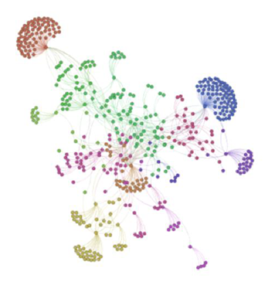
In many networks—social networks, electrical power networks, networks of web pages, etc.—the number of connections for each node follows a statistical distribution known as a power law. Here’s a model of network formation that shows how power laws can emerge from very simple rules.

Albert-László Barabási describes the following algorithm in his book Linked. Create a network by starting with two connected nodes. Then add nodes one at a time. Every time a new node joins the network, it connects to two older nodes at random with probability proportional to the number of links the old nodes have. That is, nodes that already have more links are more likely to get new links. If a node has three times as many links as another node, then it’s three times as attractive to new nodes. The rich get richer, just like with Page Rank.

Barabási says this algorithm produces networks whose connectivity distribution follows a power law. That is, the number of nodes with n connections is proportional to nk. In particular he says k = 3.

I wrote some code to play with this algorithm. As the saying goes, programming is understanding. There were aspects of the algorithm I never would have noticed had I not written code for it. For one thing, after I decided to write a program I had to read the description more carefully and I noticed I’d misunderstood a couple details.

If the number of nodes with n connections really is proportional to nk, then when you plot the number of nodes with 1, 2, 3, … connections, the points should fall near a straight line when plotted on the log-log scale and the slope of this line should be –k.

In my experiment with 10,000 nodes, I got a line of slope −2.72 with a standard error of 0.04. Not exactly −3, but maybe the theoretical result only holds in the limit as the network becomes infinitely large. The points definitely fall near a straight line in log-log scale:

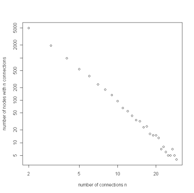
In this example, about half the nodes (5,073 out of 10,000) had only two connections. The average number of connections was 4, but the most connected node had 200 connections.

Note that the number of connections per node does not follow a bell curve at all. The standard deviation on the number of connections per node was 6.2. This means the node with 200 connections was over 30 standard deviations from the average. That simply does not happen with normal (Gaussian) distributions. But it’s not unusual at all for power law distributions because they have such thick tails.

Of course real networks are more complex than the model given here. For example, nodes add links over time, not just when they join a network. Barabási discusses in his book how some elaborations of the original model still produce power laws (possibly with different exponents) and while others do not.