Non-associative multiplication

There are five ways to parenthesize a product of four things:

  • ((ab)c)d
  • (ab)(cd)
  • (a(b(cd))
  • (a(bc))d
  • (a((bc)d)

In a context where multiplication is not associative, the five products above are not necessarily the same. Maybe all five are different.

This post will give two examples where the products above are all different: octonions and matrix multiplication.

If you’re thinking “But wait: matrix multiplication is associative!” then read further and see in what sense I’m saying it’s not.

Octonions

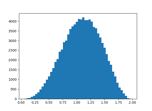
Octonion multiplication is not associative. I wrote a blog post a while back asking how close the octonions come to being associative. That is, if we randomly generate unit-length octonions a, b, and c, we can calculate the norm of

(ab)ca(bc)

and ask about its expected value. Sometimes for a triple of octonions this value is zero, but on average this expression has norm greater than 1. I estimated the average value via simulation, and later Greg Egan worked out the exact value. His write-up had gone down with the Google+ ship, but recently Greg posted a new version of his notes.

In this post I gave Python code for multiplying octonions using a function called CayleyDickson named after the originators of the algorithm. Let’s rename it m to have something shorter to work with and compute all five ways of associating a product of four octonions.

    import numpy as np

    def m(x, y):
        return CayleyDickson(x, y)

    def take_five(a, b, c, d):
        return [
            m(a, (m(b, m(c, d)))),
            m(m(a, b), m(c, d)),
            m(m(m(a, b), c), d),
            m(a, m(m(b, c), d)),
            m(m(a, m(b, c)), d)
    ]

I first tried products of basis elements, and I only got two different products out of the five ways of associating multiplication, but I only tried a few examples. However, when I tried using four random octonions, I got five different products.

    np.random.seed(20220201)

    a = np.random.rand(8)
    b = np.random.rand(8)
    c = np.random.rand(8)
    d = np.random.rand(8)

    for t in take_five(a, b, c, d):
        print(t)

This gave a very interesting result: I got five different results, but only two different real (first) components. The five vectors all differed in the last seven components, but only produced two distinct first components.

    [ 2.5180856  -2.61618184  ...]
    [ 2.5180856   0.32031027  ...]
    [ 2.5180856   1.13177500  ...]
    [ 3.0280984  -0.30169446  ...]
    [ 3.0280984  -2.36523580  ...]

I repeated this experiment a few times, and the first three results always had the same real component, and the last two results had another real component.

I suspect there’s a theorem that says

Re( ((ab)c)d ) = Re( (ab)(cd) ) = Re( a(b(cd)) )

and

Re( (a(bc))d ) = Re( a((bc)d) )

but I haven’t tried to prove it. If you come with a proof, or a counterexample, please post a link in the comments.

Matrix multiplication

Matrix multiplication is indeed associative, but the efficiency of matrix multiplication is not. That is, any two ways of parenthesizing a matrix product will give the same final matrix, but the cost of the various products are not the same. I first wrote about this here.

This is a very important result in practice. Changing the parentheses in a matrix product can make the difference between a computation being practical or impractical. This comes up, for example, in automatic differentiation and in backpropagation for neural networks.

Suppose A is an m by n matrix and B is an n by p matrix. Then AB is an m by p matrix, and forming the product AB requires mnp scalar multiplications. If C is a by q matrix, then (AB)C takes

mnp + mpq = mp(n + q)

scalar multiplications, but computing A(BC) takes

npqmnq = nq(m + p)

scalar multiplications, and in general these are not equal.

Let’s rewrite our multiplication function m and our take_five function to compute the cost of multiplying four matrices of random size.

We’ve got an interesting programming problem in that our multiplication function needs to do two different things. First of all, we need to know the size of the resulting matrix. But we also want to keep track of the number of scalar multiplications the product would require. We have a sort of main channel and a side channel. Having our multiplication function return both the dimension and the cost would make composition awkward.

This is kind of a fork in the road. There are two ways to solving this problem, one high-status and one low-status. The high-status approach would be to use a monad. The low-status approach would be to use a global variable. I’m going to take the low road and use a global variable. What’s one little global variable among friends?

    mults = 0

    def M(x, y):
        global mults
        mults += x[0]*x[1]*y[0]
        return (x[0], y[1])

    def take_five2(a, b, c, d):

        global mults
        costs = []

        mults = 0; M(a, (M(b, M(c, d)))); costs.append(mults)
        mults = 0; M(M(a, b), M(c, d));   costs.append(mults)
        mults = 0; M(M(M(a, b), c), d);   costs.append(mults)
        mults = 0; M(a, M(M(b, c), d));   costs.append(mults)
        mults = 0; M(M(a, M(b, c)), d);   costs.append(mults)

        return costs 

Next, I’ll generate five random integers, and group them in pairs as sizes of matrices conformable for multiplication.

    dims = np.random.random_integers(10, size=5)
    dim_pairs = zip(dims[:4], dims[1:])
    c = take_five2(*[p for p in dim_pairs])

When I ran this dims was set to

[3 9 7 10 6]

and so my matrices were of size 3×9, 9×7, 7×10, and 10×6.

The number of scalar multiplications required by each way of multiplying the four matrices, computed by take_five2 was

[1384, 1090, 690, 1584, 984]

So each took a different number of operations. The slowest approach would take more than twice as long as the fastest approach. In applications, matrices can be very long and skinny, or very wide and thin, in which case one approach may take orders of magnitude more operations than another.

Related posts

Conjugate theorem for octonions

Yesterday I wrote about the fact that quaternions, unlike complex numbers, can form conjugates via a series of multiplications and additions. This post will show that you can do something similar with octonions.

If x is an octonion

x = r0 e0 + r1 e1 + … + r7 e7

where all the r‘s are real numbers. The conjugate flips the signs of all the components except the real component:

x* = r0 e0r1 e1 − … − r7 e7

The conjugate theorem says

x* = − (x + (e1 x) e1 + … + (e7 x) e7) / 6

which is analogous to the theorem

q* = − (q + iqi + jqj + kqk) /2

for quaternions.

The internal parentheses are necessary because multiplication in octonions is not associative:

xyz

is ambiguous because it could mean

(xy)z

or

x(yz)

and the two are not necessarily equal.

Update: It is true in general that (xy)zx(yz) for octonions. However, the subalgebra of octonions generated by any two elements is associative. In particular, (xy)xx(yz) and so we can write the equation for x* above as simply

x* = − (x + e1 x e1 + … + e7 x e7) / 6.

Thanks to Martin Erik Horn for pointing this out.

The proof is also analogous to the proof given in the earlier post for quaternions. First work out what the effect is of multiplying on the left and right by one of the imaginary units, then add everything up. You’ll find that the real component is multiplied by -6 and the rest of the components are multiplied by 6.

How to multiply octonions

This post will present a way of multiplying octonions that’s easy to remember.

Please note that there are varying conventions for how to define multiplication for octonions [1].

Octonions

The complex numbers have one imaginary unit i, and the quaternions have three: i, j, and k. The octonions have seven, and so it makes sense to switch over to subscripts rather than venturing further out into the alphabet. Besides, numerical indices will be useful for reasons we’ll see shortly.

Let e0 = 1 and let e1 through e7 be the imaginary units for octonions. Then the e‘s form a basis for ℝ8. The octonions are ℝ8 with a product that distributes over addition, but the product is not commutative or associative.

Multiplication is determined by how the basis elements multiply, and there are multiple ways of presenting these multiplication rules, the simplest being to write down a multiplication table. Here I’ll present the way I find easiest to remember [2].

Multiplication rules

The squares of each of the imaginary units e1 through e7 are equal to −1, as you’d expect based on experience with complex numbers and quaternions. You can derive the rest of the multiplication facts from

e1 e2 = e4

and two simple rules.

The first rule is that the equation above holds when you shift the indices mod 7.

e1 e2 = e4
e2 e3 = e5
e3 e4 = e6
e4 e5 = e7
e5 e6 = e1
e6 e7 = e2
e7 e1 = e3

The second rule is that each of the triplets of units above behave analogous to i, j, and k in quaternions. That is, when you take a triple like (e2, e3, e5), rotations don’t flip the sign but swapping adjacent elements does. That is,

e2 e3 = e5
e5 e2 = e3
e3 e5 = e2

and

e3 e2 = −e5
e2 e5 = −e3
e5 e3 = −e2

So we have seven rotations of the equation

e1 e2 = e4

and six permutations of each rotation, for a total of 42 rules. We already had 7 rules, saying each unit squares to -1, so we have the 49 rules we need to multiply all the non-real units by each other.

More octonion posts

[1] There are multiple conventions for defining octonion multiplication. For example, according to a common definition,

e1 e2 = e3

but according to our definition

e1 e2 = e4

In fact, there are 480 ways to define the multiplication rules for e1 through e7. However, all the ways of defining octonion multiplication are isomorphic. You can translate results from one convention to another by renumbering the basis elements. For example, you can convert from the first convention above to our convention by relabeling

(e1, e2, e3, e4, e5, e6, e7)

as

(e1, e2, e4, – e7, e3, e6, e5).

I picked the convention used here because it makes the multiplication rules easy to remember: the mod 7 rule doesn’t hold for some other ways of defining multiplication.

[2] There’s a neat way of representing octonion multiplication rules in terms of a Fano plane diagram, but to use it you have to remember how to label the diagram. The presentation in this post is easier to remember, in my opinion. You might remember the rules given here, then use them to fill in a Fano diagram.

Complex Conjugates versus Quaternion Conjugates

The conjugate of a complex number

z = a + bi

is the complex number

z^* = a - bi

Taking the conjugate flips over a complex number, taking its reflection in the real axis.

Multiplication stretches and rotates complex numbers, and addition translates complex numbers. You can’t flip the complex plane over by any series of dilatations, rotations, and translations.

The situation is different for quaternions. The conjugate of a quaternion

q = a + bi + cj + dk

is

q^* = a - bi - cj - dk

You can flip four dimensional space over by a series of dilations, rotations, and translations. Namely

q^* = -\frac{1}{2}(q + iqi + jqj + kqk)

To prove this equation, let’s first see what happens when you multiply q on both sides by i:

i(a + bi + cj + dk)i = -a - bi + cj + dk

That is, the effect of multiplying on both sides by i is to flip the sign of the real component and the i component.

Multiplying on both sizes by j or k works analogously: it flips the sign of the real component and its component, and leaves the other two alone.

It follows that

\begin{align*} q +iqi + jqj + kqk &= \phantom{-}a + bi + cj +dk \\ & \,\phantom{=} - a - bi + cj + dk \\ & \,\phantom{=} - a + bi - cj + dk \\ & \,\phantom{=} - a + bi + cj - dk \\ &= -2a + 2bi + 2cj + 2dk\\ &= -2q^* \end{align*}

and so the result follows from dividing by −2.

Update: There’s an analogous theorem for octonions.

More on quaternions

How close is octonion multiplication to being associative?

Quaternion multiplication is associative but not commutative. An earlier post looked at the average size of the commutator xyyx as a measure of how far quaternion multiplication is from being commutative.

This post looks at an analogous question for octonions. Octonion multiplication is neither commutative nor associative. So in this post we look at the associator of three octonions (xy)zx(yz) as a measure of how far octonion multiplication is from being associative.

(A post from yesterday looked at how close octonion multiplication comes to being associative in an algebraic sense, looking at weak forms of associativity. This post looks at how close multiplication comes to being associative in an analytical sense, looking at norm distances rather than algebraic identities.)

We will use a simulation to look at the average norm of the octonion associator over the octonions of unit length, analogous to the earlier post that looked at the commutator of the quaternions. We developed code for octonion multiplication in the previous post and will reuse that code here. We also developed code for generating random unit-length octonions in the same post.

Here’s code to find the average norm of the associator and plot a histogram of its values.

    
    import matplotlib.pyplot as plt

    # omult is octonion multiplication. 
    # See previous post.
    def associator(x, y, z):
        return omult(omult(x, y), z) - 
               omult(x, omult(y, z))

    N = 100000
    s = 0
    h = np.zeros(N)
    for n in range(N):
        x = random_unit_octonion()
        y = random_unit_octonion()
        z = random_unit_octonion()    
        t = norm(associator(x, y, z))
        s += t
        h[n] = t

    print(s/N)
    plt.hist(h, bins=50)
    plt.show()

This gives an average of 1.095 and the histogram below.

histogram of octonion associator norm values

Update: Greg Egan calculated the exact mean value for the norm of the associator to be 147456/(42875 π) ≈ 1.0947336. Here are the details.

Python code for octonion and sedenion multiplication

The previous post discussed octonions. This post will implement octonion multiplication in Python, and then sedenion multiplication.

Cayley-Dickson construction

There’s a way to bootstrap quaternion multiplication into octonion multiplication, so we’ll reuse the quaternion multiplication code from an earlier post. It’s called the Cayley-Dickson construction. For more on this construction , see John Baez’s treatise on octonions.

If you represent an octonion as a pair of quaternions, then multiplication can be defined by

(a, b) (c, d) = (acd*b, da + bc*)

where a star superscript on a variable means (quaternion) conjugate.

Note that this isn’t the only way to define multiplication of octonions. There are many (480?) isomorphic ways to define octonion multiplication.

(You can take the Cayley-Dickson construction one step further, creating sedenions as pairs of octonions. We’ll also provide code for sedenion multiplication below.)

Code for octonion multiplication

    import numpy as np

    # quaternion multiplication
    def qmult(x, y):
        return np.array([
            x[0]*y[0] - x[1]*y[1] - x[2]*y[2] - x[3]*y[3],
            x[0]*y[1] + x[1]*y[0] + x[2]*y[3] - x[3]*y[2],
            x[0]*y[2] - x[1]*y[3] + x[2]*y[0] + x[3]*y[1],
            x[0]*y[3] + x[1]*y[2] - x[2]*y[1] + x[3]*y[0]
       ])

    # quaternion conjugate
    def qstar(x):
        return x*np.array([1, -1, -1, -1])

    # octonion multiplication
    def omult(x, y):
        # Split octonions into pairs of quaternions
        a, b = x[:4], x[4:]
        c, d = y[:4], y[4:]
    
        z = np.zeros(8)
        z[:4] = qmult(a, c) - qmult(qstar(d), b)
        z[4:] = qmult(d, a) + qmult(b, qstar(c))
        return z

Update: See this post for refactored code. Handles quaternions, octonions, sedenions, etc. all with one function.

Unit tests

Here are some unit tests to verify that our multiplication has the expected properties. We begin by generating three octonions with norm 1.

    from numpy.linalg import norm

    def random_unit_octonion():
        x = np.random.normal(size=8)
        return x / norm(x)

    x = random_unit_octonion()
    y = random_unit_octonion()
    z = random_unit_octonion()

We said in the previous post that octonions satisfy the “alternative” condition, a weak form of associativity. Here we verify this property as a unit test.

    eps = 1e-15

    # alternative identities

    a = omult(omult(x, x), y)
    b = omult(x, omult(x, y))
    assert( norm(a - b) < eps )

    a = omult(omult(x, y), y)
    b = omult(x, omult(y, y))
    assert( norm(a - b) < eps )

We also said in the previous post that the octonions satisfy the “Moufang” conditions.

    # Moufang identities
    
    a = omult(z, omult(x, omult(z, y)))
    b = omult(omult(omult(z, x), z), y)
    assert( norm(a - b) < eps )

    a = omult(x, omult(z, omult(y, z)))
    b = omult(omult(omult(x, z), y), z)
    assert( norm(a - b) < eps )

    a = omult(omult(z,x), omult(y, z))
    b = omult(omult(z, omult(x, y)), z)
    assert( norm(a  - b) < eps )

    a = omult(omult(z,x), omult(y, z))
    b = omult(z, omult(omult(x, y), z))
    assert( norm(a - b) < eps )

And finally, we verify that the product of unit length octonions has unit length.

    # norm condition
    n = norm(omult(omult(x, y), z))
    assert( abs(n - 1) < eps )

The next post uses the octonion multiplication code above to look at the distribution of the associator (xy)z – x(yz) to see how far multiplication is from being associative.

Sedenion multiplication

The only normed division algebras over the reals are the real numbers, complex numbers, quaternions, and octonions. These are real vector spaces of dimension 1, 2, 4, and 8.

You can proceed analogously and define a real algebra of dimension 16 called the sedenions. When we go from complex numbers to quaternions we lose commutativity. When we go from quaternions to octonions we lose full associativity, but retain a weak version of associativity. Even weak associativity is lost when we move from octonions to sedenions.  Non-zero octonions form an alternative loop with respect to multiplication, but sedenions do not.

Sedenions have multiplicative inverses, but there are also some zero divisors, i.e. non-zero vectors whose product is zero. So sedenions do not form a division algebra. If you continue the Cayley-Dickson construction past the sedenions, you keep getting zero divisors, so no more division algebras.

Here’s Python code for sedenion multiplication, building on the code above.

    def ostar(x):
        mask = -np.ones(8)
        mask[0] = 1
        return x*mask
 
    # sedenion multiplication
    def smult(x, y):
        # Split sedenions into pairs of octonions
        a, b = x[:8], x[8:]
        c, d = y[:8], y[8:]
        z = np.zeros(16)
        z[:8] = omult(a, c) - omult(ostar(d), b)
        z[8:] = omult(d, a) + omult(b, ostar(c))
        return z

As noted above, see this post for more concise code that also generalizes further.

Fibonacci number system

Every positive integer can be written as the sum of distinct Fibonacci numbers. For example, 10 = 8 + 2, the sum of the fifth Fibonacci number and the second.

This decomposition is unique if you impose the extra requirement that consecutive Fibonacci numbers are not allowed. [1] It’s easy to see that the rule against consecutive Fibonacci numbers is necessary for uniqueness. It’s not as easy to see that the rule is sufficient.

Every Fibonacci number is itself the sum of two consecutive Fibonacci numbers—that’s how they’re defined—so clearly there are at least two ways to write a Fibonacci number as the sum of Fibonacci numbers, either just itself or its two predecessors. In the example above, 8 = 5 + 3 and so you could write 10 as 5 + 3 + 2.

The nth Fibonacci number is approximately φn/√5 where φ = 1.618… is the golden ratio. So you could think of a Fibonacci sum representation for x as roughly a base φ representation for √5x.

You can find the Fibonacci representation of a number x using a greedy algorithm: Subtract the largest Fibonacci number from x that you can, then subtract the largest Fibonacci number you can from the remainder, etc.

Programming exercise: How would you implement a function that finds the largest Fibonacci number less than or equal to its input? Once you have this it’s easy to write a program to find Fibonacci representations.

* * *

[1] This is known as Zeckendorf’s theorem, published by E. Zeckendorf in 1972. However, C. G. Lekkerkerker had published the same result 20 years earlier.