Approximating a solution that doesn’t exist

Posted on 11 August 2009 by John

The following example made an impression on me when I first saw it years ago. I still think it’s an important example, though I’d draw a different conclusion from it today.

Problem: Let y(t) be the solution to the differential equation y‘ = t² + y² with y(0) = 1. Calculate y(1).

If we use Euler’s numerical method with a step size h = 0.1, we get y(1) = 7.19. If we reduce the step size to 0.05 we get y(1) = 12.32. If we reduce the step size further to 0.01, we get y(1) = 90.69. That’s strange. Let’s switch over to a more accurate method, 4th order Runge-Kutta. With a step size 0.1 the Runge-Kutta method gives 735.00, and if we use a step size of 0.01 we get a result larger than 10¹⁵. What’s going on?

The problem presupposes that a solution exists at t = 1 when in fact no solution exists. General theory (Picard’s theorem) tells that a unique solution exists for some interval containing 0, but it does not tell us how far that interval extends. With a little work we can show that a solution exists for t at least as large as π/4. However, the solution becomes unbounded somewhere between π/4 and 1.

When I first saw this example, my conclusion was that it showed how important theory is. If you just go about numerically computing solutions without knowing that a solution exists, you can think you have succeeded when you’re actually computing something that doesn’t exist. Prove existence and uniqueness before computing. Theory comes first.

Now I think the example shows the importance of the interplay between theory and numerical computation. It would be nice to know how big the solution interval is before computing anything, but that’s not always possible. Also, it’s not obvious from looking at the equation that there should be a problem at t = 1. The difficulties we had with numerical computation suggested there might be a theoretical problem.

I first saw this problem in an earlier edition of Boyce and DiPrima. The book goes on to approximate the interval over which the solution does exist using a combination of analytical and numerical methods. It looks like the solution becomes unbounded somewhere near t = 0.97.

I wouldn’t say that theory or computation necessarily come first. I’d say you iterate between them, starting with the approach that is more tractable. Theoretical results are more satisfying when they’re available, but theory often doesn’t tell us as much as we’d like to know. Also, people make mistakes in theoretical computation just as they do in numerical computation. It’s best when theory and numerical work validate each other.

The problem does show the importance of being concerned with existence and uniqueness, but theoretical methods are not the only methods for exploring existence. Good numerical practice, i.e. trying more than one step size or more than one numerical method, is also valuable. In any case, the problem shows that without some diligence — either theoretical or numerical — you could naively compute an approximate “solution” where no solution exists.

Anatomy of a floating point number

Posted on 6 April 2009 by John

In my previous post, I explained that floating point numbers are a leaky abstraction. Often you can pretend that they are mathematical real numbers, but sometimes you cannot. This post peels back the abstraction and explains exactly what a floating point number is. (Technically, this post describes an IEEE 754 double precision floating point number, by far the most common kind of floating point number in practice.)

A floating point number has 64 bits that encode a number of the form ± p × 2^e. The first bit encodes the sign, 0 for positive numbers and 1 for negative numbers. The next 11 bits encode the exponent e, and the last 52 bits encode the precision p. The encoding of the exponent and precision require some explanation.

The exponent is stored with a bias of 1023. That is, positive and negative exponents are all stored in a single positive number by storing e + 1023 rather than storing e directly. Eleven bits can represent integers from 0 up to 2047. Subtracting the bias, this corresponds to values of e from −1023 to +1024. Define e_min = −1022 and e_max = +1023. The values e_min − 1 and e_max + 1 are reserved for special use. More on that below.

Floating point numbers are typically stored in normalized form. In base 10, a number is in normalized scientific notation if the significand is ≥ 1 and < 10. For example, 3.14 × 10² is in normalized form, but 0.314 × 10³ and 31.4 × 10² are not. In general, a number in base β is in normalized form if it is of the form p × β^e where 1 ≤ p < β. This says that for binary, i.e. β = 2, the first bit of the significand of a normalized number is always 1. Since this bit never changes, it doesn’t need to be stored. Therefore we can express 53 bits of precision in 52 bits of storage. Instead of storing the significand directly, we store f, the fractional part, where the significand is of the form 1.f.

The scheme above does not explain how to store 0. Its impossible to specify values of f and e so that 1.f × 2^e = 0. The floating point format makes an exception to the rules stated above. When e = e_min − 1 and f = 0, the bits are interpreted as 0. When e = e_min − 1 and f ≠ 0, the result is a denormalized number. The bits are interpreted as 0.f × 2^e_min. In short, the special exponent reserved below e_min is used to represent 0 and denormalized floating point numbers.

The special exponent reserved above e_max is used to represent ∞ and NaN. If e = e_max + 1 and f = 0, the bits are interpreted as ∞. But if e = e_max + 1 and f ≠ 0, the bits are interpreted as a NaN or “not a number.” See IEEE floating point exceptions for more information about ∞ and NaN.

Since the largest exponent is 1023 and the largest significant is 1.f where f has 52 ones, the largest floating point number is

2¹⁰²³(2 − 2⁻⁵²) = 2¹⁰²⁴ − 2⁹⁷¹ ≈ 2¹⁰²⁴ ≈ 1.8 × 10³⁰⁸.

In C, this constant is defined as DBL_MAX, defined in <float.h>.

Since the smallest exponent is -1022, the smallest positive normalized number is 1.0 × 2⁻¹⁰²² ≈ 2.2 × 10⁻³⁰⁸. In C, this is defined as DBL_MIN. However, it is not the smallest positive number representable as a floating point number, only the smallest normalized floating point number. Smaller numbers can be expressed in denormalized form, albeit at a loss of significance. The smallest denormalized positive number occurs with f has 51 0’s followed by a single 1. This corresponds to 2⁻⁵²*2⁻¹⁰²² = 2⁻¹⁰⁷⁴ ≈ 4.9 × 10⁻³²⁴. Attempts to represent any smaller number must underflow to zero.

C gives the name DBL_EPSILON to the smallest positive number ε such that 1 + ε ≠ 1 to machine precision. Since the significant has 52 bits, it’s clear that DBL_EPSILON = 2⁻⁵² ≈ 2.2 × 10⁻¹⁶. That is why we say a floating point number has between 15 and 16 significant (decimal) figures.

For more details see What Every Computer Scientist Should Know About Floating-Point Arithmetic.

First post in this series: Floating point numbers are a leaky abstraction

Floating point numbers are a leaky abstraction

Posted on 6 April 2009 by John

Joel Spolsky coined the term leaky abstraction for programming concepts that usually shield you from messy details but sometimes break down. A perfect abstraction is a black box that you never have to open. A leaky abstraction is a black box that you have to open up occasionally.

Floating point numbers, the computer representations of real numbers, are leaky abstractions. They work remarkably well: you can usually pretend that a floating point type is a mathematical real number. But sometimes you can’t. The abstraction leaks, though not very often.

Most explanations I’ve heard for the limitations of machine numbers are pedantic. “There are only a finite number of floating point numbers so they can’t represent real numbers well.” That’s not much help. It doesn’t explain why floating point numbers actually do represent real numbers sufficiently well for most applications, and it doesn’t suggest where the abstraction might leak.

A standard floating point number has roughly 16 decimal places of precision and a maximum value on the order of 10³⁰⁸, a 1 followed by 308 zeros. (According to IEEE standard 754, the typical floating point implementation.)

Sixteen decimal places is a lot. Hardly any measured quantity is known to anywhere near that much precision. For example, the constant in Newton’s Law of Gravity is only known to six significant figures. The charge of an electron is known to 11 significant figures, much more precision than Newton’s gravitational constant, but still less than a floating point number. So when are 16 figures not enough? One problem area is subtraction. The other elementary operations — addition, multiplication, division — are very accurate. As long as you don’t overflow or underflow, these operations often produce results that are correct to the last bit. But subtraction can be anywhere from exact to completely inaccurate. If two numbers agree to n figures, you can lose up to n figures of precision in their subtraction. This problem can show up unexpectedly in the middle of other calculations. For an example, see this post on calculating standard deviation.

What about overflow or underflow? When do you need numbers bigger than 10³⁰⁸? Often you don’t. But in probability calculations, for example, you need them all the time unless you’re clever. It’s common in probability to compute a medium-sized number that is the product of an astronomically large number and an infinitesimally small number. The final result fits into a computer just fine, but the intermediate numbers might not due to overflow or underflow. For example, the maximum floating point number on most computers is somewhere between 170 factorial and 171 factorial. Such large factorials often appear in applications, often in ratios with other large factorials.

Often you can afford to be blissfully ignorant of the details of floating point arithmetic, but sometimes you cannot. A great place to learn more is David Goldberg’s paper What Every Computer Scientist Should Know About Floating-Point Arithmetic.

Update: See follow-up post, Anatomy of a floating point number.

Interpolation errors

Posted on 1 April 2009 by John

Say you have a function f(x) and you want to find a polynomial p(x) that agrees with f(x) at several points. Given a set of points

x₀, x₁, x₂, …, x_n

you can always find a polynomial of degree n such that p(x_i) = f(x_i) for i = 0, 1, 2, …, n. It seems reasonable that the more points you pick, the better the interpolating polynomial p(x) will match the function f(x). If the two functions match exactly at a lot of points, they should match well everywhere. Sometimes that’s true and sometimes it’s not.

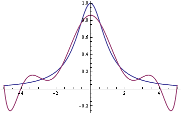
Here is a famous example due to Carle Runge. Let f(x) = 1/(1 + x²) and let p_n be the polynomial that interpolates f(x) at n+1 evenly spaced nodes in the interval [−5, 5]. As n becomes larger, the fit becomes worse.

Here’s a graph of f(x) and p₉(x). The smooth blue line is f(x) and the wiggly red line is p₉(x).

graph of f(x) and p9(x)

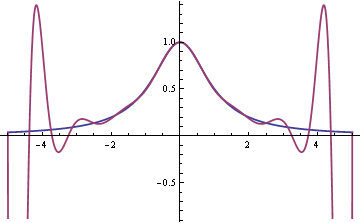
Here’s the analogous graph for p₁₆(x).

graph of f(x) and p16(x)

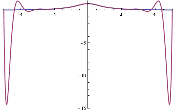
The fit is improving in the middle. In fact, the curves agree to within the thickness of the plot line from say −1 to 1. But the fit is so bad in the tails that the graph had to be cut off. Here’s another plot of f(x) and p₁₆(x) on a different scale to show how far negative the polynomial dips.

graph of f(x) and p16(x) on different scale

The problem is the spacing of the nodes. Interpolation errors are bad for evenly spaced nodes.

Update: This post explains in a little more depth why this particular function has problems and gives another example where interpolation at evenly-spaced nodes behaves badly.

If we interpolate f(x) at different points, at the Chebyshev nodes, then the fit is good.

interpolating at Chebyshev nodes

The Chebyshev nodes on [−1, 1] are x_i = cos( π i / n ). Here we multiplied these nodes by 5 to scale to the interval [−-5, 5].

If the function f(x) is absolutely continuous, as in our example, then the interpolating polynomials converge uniformly when you interpolate at Chebyshev nodes. However, ordinary continuity is not enough. Given any sequence of nodes, there exists a continuous function such that the polynomial interpolation error grows like log(n) as the number of nodes n increases.

Some numerical integration methods are based on interpolating polynomials: fit a polynomial to the integrand, then integrate the polynomial exactly to approximate the original integral. The examples above suggest that increasing the order of such integration methods might not improve accuracy and might even make things worse.

Related: Need help with interpolation?

Quasi-random sequences in art and integration

Posted on 16 March 2009 by John

Sometimes when people say they want random points, that’s not what they really want. Random points clump more than most people expect. Quasi-random sequences are not random in any mathematical sense, but they might match popular expectations of randomness better than the real thing, especially for aesthetic applications. If by “random” someone means “scattered around without a clear pattern and not clumped together” then quasi-random sequences might do the trick.

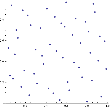
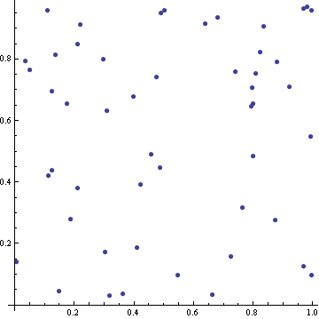
Here are the first 50 points in a quasi-random sequence of points in the unit square.

quasi-random points

By contrast, here are 50 points in a unit square whose coordinates are uniform random samples.

random points

The truly random points clump together. Notice the cluster of three points in the top right corner. There are few other instances of pairs of points being very close together. Also, there are fairly large areas that don’t contain any random points. The quasi-random points by contrast are better spread out. They have a self-avoiding property that keeps them from clustering, and they fill the space more efficiently.

Quasi-random sequences could be confused with pseudo-random sequences. They’re not at all the same thing. Pseudo-random sequences are computer-generated sequences that in many ways behave as if they were truly random, even though they were produced by deterministic algorithms. For many practical purposes, including sensitive statistical tests, pseudo-random sequences are simply random sequences. (The “truly” random points above were technically “pseudo-random” points.)

The quasi-random points above were part of a Sobol sequence, a common quasi-random sequence. Other quasi-random sequences include the Halton sequence and the Hammersley sequence. Mathematically, these sequences are defined has having low-discrepancy. Roughly speaking, this means the “discrepancy” between the number of points that actually fall in a volume and the number of points you’d expect to fall in the same volume is small. See the Wikipedia article on quasi-random sequences for more mathematical details.

Besides being aesthetically useful, quasi-random sequences are useful in applied mathematics. Because these sequences explore a space more efficiently than random sequences, quasi-random sequences sometimes lead to more efficient high-dimensional integration algorithms than Monte Carlo integration. Quasi-Monte Carlo integration, i.e. integration based on quasi-random sequences rather than random sequences, is popular in financial applications. Art Owen has written insightful papers on Quasi-Monte Carlo integration (QMC). He has classified which integration problems can be efficiently computed via QMC methods and which cannot. In a nutshell, QMC works well when the effective dimension of a problem is significantly lower than the actual dimension. For example, a financial model might ostensibly depend on 1000 variables, but 50 of those variables contribute far more to the integrand than all the other variables. The integrand might essentially be a function of only 50 variables. In that case, QMC will work well. Note that it is not necessary to identify these 50 variables or do any change of variables. QMC just magically takes advantage of the situation.

One disadvantage of QMC integration is that it doesn’t naturally lead to an estimate of its own accuracy, unlike Monte Carlo integration. Several hybrid approaches have been proposed to combine QMC integration and Monte Carlo integration to get the efficiency of the former and the error estimates of the latter. For example, one could randomly jitter the quasi-random points or randomly permute their components. Some of these results are in Art Owen’s papers.

To read more about quasi-random sequences, see the book Random Number Generation and Quasi-Monte Carlo Methods.

The smoothest curve through a set of points

Posted on 6 February 2009 by John

How do you fit the smoothest curve through a set of points? Suppose you have a set of increasing x values x₁, x₂, x₃, … , x_n and a corresponding set of y values y₁, y₂, y₃, … , y_n. You want to find the smoothest function f(x) such that f(x_i) = y_i for i = 1, 2, 3, …, n. The smoothest curve depends on how you define smoothness, but we’ll develop a common definition that leads to a nice solution.

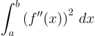
Our definition of smoothness starts with the second derivative. If a curve is flat, it has zero second derivative. If the curve has a sharp kink, the second derivative will be high there. We want to add up the smoothness over the entire curve, so we’ll integrate the second derivative. But that won’t quite work. Second derivatives can be positive or negative, and a curve could have several sharp bends and still have average second derivative zero. Sharp bends in one direction could be canceled out by equally sharp bends in the opposite direction. So we look at the square of the second derivative. That gives a positive number whether the curve bends up or down. Also, squaring small numbers makes them smaller and squaring big numbers makes them bigger. So squaring the second derivative will penalize sharp bends and be more forgiving of small bends. In summary, we’ll measure the smoothness of a function f(x) over an interval [a, b] by the following integral.

$\int_a^b \left( f''(x) \right)^2\, dx$

Using the above measure of smoothness, the smoothest function interpolating a set of values is a natural cubic spline. I’ll explain this definition from right to left: first I’ll explain what a spline is, then a cubic spline, then a natural cubic spline. Cubic splines are very commonly used in graphical applications.

A spline is a function made by piecing together other functions. Most splines are piecewise polynomials, though there are other kinds of splines, such as trigonometric splines that are piecewise trig functions. The term “spline” comes from a mechanical device for drawing curves.

A cubic spline is formed by piecing together cubic polynomials. That is, the restriction of f to any interval between two x-values, from x_i to x_i+1 is a cubic polynomial. These piecewise cubic polynomials are formed by making their first and second derivatives match where they join. This makes a cubic spline curve appear very smooth.

Say we have n values of x and y. That means we have n − 1 cubic polynomials to fit together: one over [x₁, x₂], another over [x₂, x₃], etc. Each cubic polynomial has 4 coefficients, and so we have a total of 4(n − 1) coefficients to determine. At each interior node, i.e. the values from x₂ to x_n-1, there are four constraints. At each such x_i we have

The polynomial on the left side must have value y_i.
The polynomial on the right side must have value y_i.
The first derivatives of the left and right polynomials must match.
The second derivatives of the left and right polynomials must match.

This gives us a total of 4(n − 2) interior constraints. The values at the left and right ends are specified too, i.e. f(x₁) = y₁ and f(x_n) = y_n. This adds up to 4n-6 constraints on 4n − 4 coefficients. We need two more constraints to have as many equations as unknowns. There are various ways to add these constraints but a natural cubic spline imposes the requirement that the second derivatives should be zero at the ends, i.e. f”(x₁) = f”(x_n) = 0.

Finding the coefficients for a natural cubic spline with n nodes requires solving 4n − 4 equations in as many unknowns. There is a unique solution to this system of equations, and the system has a special structure that can be solved very quickly.

One thing I find interesting about natural cubic splines is how a fairly ad hoc procedure — patching cubic polynomials — leads to the solution to an elegant minimization problem.

Related: Help with interpolation

Convex optimization

Posted on 7 January 2009 by John

I’ve enjoyed following Stephen Boyd’s lectures on convex optimization. I stumbled across a draft version of his textbook a few years ago but didn’t realize at first that the author and the lecturer were the same person. I recommend the book, but I especially recommend the lectures. My favorite parts of the lectures are the off-hand remarks about which methods are well known and which are not, what different fields call the same methods, which concerns are merely academic minutia and which are practically important. This kind of information is almost impossible to pick up just from reading books and articles.

A surprisingly large set of problems can be formulated as minimizing a convex function subject to convex constraints, and algorithms for solving these problems are very well developed. It’s roughly true that an optimization problem is tractable if and only if it is convex. Of course that’s not exactly true. Many special non-convex problems can be solved easily, though if you write down an arbitrary non-convex optimization problem, it’s probably hard to solve. On the other hand, enormous convex optimization problems can often be solved quite efficiently.

I became interested in optimization a few years ago in order to solve some problems that came up at work. After going through Boyd’s lectures, I’d like to go back and do a better job on some of these problems. For example, the EffTox dose-finding software solves an optimization problem to determine prior parameters based on input from doctors. That optimization is slow and not very robust. If I can find the time to do it, I think I could improve that software.

Orthogonal polynomials

Posted on 16 February 2008 by John

This morning I posted some notes on orthogonal polynomials and Gaussian quadrature.

“Orthogonal” just means perpendicular. So how can two polynomials be perpendicular to each other? In geometry, two vectors are perpendicular if and only if their dot product of their coordinates is zero. In more general settings, two things are said to be orthogonal if their inner product (generalization of dot product) is zero. So what was a theorem in basic geometry is taken as a definition in other settings. Typically mathematicians say “orthogonal” rather than “perpendicular.” The basic idea of lines meeting at right angles acts as a reliable guide to intuition in more general settings.

Two polynomials are orthogonal if their inner product is zero. You can define an inner product for two functions by integrating their product, sometimes with a weighting function.

Orthogonal polynomials have remarkable properties that are easy to prove. Last week I posted some notes on Chebyshev polynomials. The notes posted today include Chebyshev polynomials as a special case and focus on the application of orthogonal polynomials to quadrature. (“Quadrature” is just an old-fashioned word for integration, usually applied to numerical integration in one dimension.) It turns out that every class of orthogonal polynomials corresponds to an integration rule.

Numerical analysis