Making a singular matrix non-singular

Posted on 13 June 2012 by John

Someone asked me on Twitter

Is there a trick to make an singular (non-invertible) matrix invertible?

The only response I could think of in less than 140 characters was

Depends on what you’re trying to accomplish.

Here I’ll give a longer explanation.

So, can you change a singular matrix just a little to make it non-singular? Yes, and in fact you can change it by as little as you’d like. Singular square matrices are an infinitely thin subset of the space of all square matrices, and any tiny random perturbation is almost certain to take you out of that thin subset. (“Almost certain” is actually a technical term here, meaning with probability 1.)

Adding a tiny bit of noise to a singular matrix makes it non-singular. But why did you want a non-singular matrix? Presumably to solve some system of equations. A little noise makes the system go from theoretically impossible to solve to theoretically possible to solve, but that may not be very useful in practice. It will let you compute a solution, but that solution may be meaningless.

A little noise makes the determinant go from zero to near zero. But here is an important rule in numerical computation:

If something is impossible at 0, it will be hard near zero.

“Hard” could mean difficult to do or it could mean the solution is ill-behaved.

Instead of asking whether a matrix is invertible, let’s ask how easy it is to invert. That is, let’s change a yes/no question into a question with a continuum of answers. The condition number of a matrix measures how easy the matrix is to invert. A matrix that is easy to invert has a small condition number. The harder it is to invert a matrix, the larger its condition number. A singular matrix is infinitely hard to invert, and so it has infinite condition number. A small perturbation of a singular matrix is non-singular, but the condition number will be large.

So what exactly is a condition number? And what do I mean by saying a matrix is “hard” to invert?

The condition number of a matrix is the norm of the matrix times the norm of its inverse. Defining matrix norms would take too long to go into here, but intuitively it is a way of sizing up a matrix. Note that you take the norm of both the matrix and its inverse. A small change to a matrix might not change its norm much, but it might change the norm of its inverse a great deal. If that is the case, the matrix is called ill-conditioned because it has a large condition number.

When I say a matrix is hard to invert, I mean it is hard to do accurately. You can use the same number of steps to invert a matrix by Gaussian elimination whether the matrix has a small condition number or a large condition number. But if the matrix has a large condition number, the result may be very inaccurate. If the condition number is large enough, the solution may be so inaccurate as to be completely useless.

You can think of condition number as an error multiplier. When you solve the linear system Ax = b, you might expect that a little error in b would result in only a little error in x. And that’s true if A is well-conditioned. But a small change in b could result in a large change in x if A is ill-conditioned. If the condition number of A is 1000, for example, the error in x will be 1000 times greater than the error in b. So you would expect x to have three fewer significant figures than b.

Note that condition number isn’t limited to loss of precision due to floating point arithmetic. If you have some error in your input b, say due to measurement error, then you will have some corresponding error in your solution to Ax = b, even if you solve the system Ax = b exactly. If the matrix A is ill-conditioned, any error in b (rounding error, measurement error, statistical uncertainty, etc.) will result in a correspondingly much larger error in x.

So back to the original question: can you make a singular matrix non-singular? Sure. In fact, it’s hard not to. Breathe on a singular matrix and it becomes non-singular. But the resulting non-singular matrix may be useless. The perturbed matrix may be theoretically invertible but practically non-invertible.

So here’s a more refined question: can you change a singular matrix into a useful non-singular matrix? Yes you can, sometimes, but the answer depends very much on the problem you’re trying to solve. This is generally known as regularization, though it goes by different names in different contexts. You use knowledge of your domain beyond the specific data at hand to guide how you change your matrix.

How to solve supposedly intractable problems

Posted on 28 February 2012 by John

Contrary to semi-educated belief, NP-complete problems are not necessarily intractable. Often such problems are intractable, but not always. If a problem is NP-complete, this means that there is no polynomial-time algorithm for solving the problem

for the worst case,
as the problem size grows,
finding exact solutions,
with certainty,
as far as anyone knows.

One way out of this (#5) is to show how to solve NP-complete problems efficiently. That may not be possible, and it hasn’t been possible so far, so we’ll not worry about this one. But that still leaves four options:

special cases
small problem sizes
approximate solutions
probabilistic solutions.

For example, the Traveling Salesman problem is NP-complete. But it’s easy to find solutions for a small number of cities by brute force. And even for a moderate number of cities, people routinely find solutions; there’s even an iPhone app for finding solutions. For larger problems, there are algorithms that yield near-optimal solutions with high probability.

Similar remarks hold for other kinds of problems deemed intractable. For example, some say you can’t find the roots of a 5th degree polynomial. Isn’t that a theorem? No. There’s a theorem that says you cannot find

exact solutions,
in general,
using a finite sequence of certain mathematical operations.

So there are three loop holes here:

approximate solutions,
special cases, and
more general operations.

If you only want to find solutions to 100 decimal places, for example, that’s doable.

Most integrals cannot be computed

by a typical calculus student,
exactly,
with certainty,
in terms of elementary functions.

But often integrals can be computed by some combination of

more sophisticated exact techniques,
numerical approximation,
randomized algorithms, and
a broader class of functions.

For example, some say that the integral of exp(-x²) cannot be computed. Of course it can, though there is not a finite combination of elementary functions that gives the exact integral. You can compute the integral exactly in terms of the error function erf(x), or compute it numerically to any desired accuracy. You could even approximate the integral with a Monte Carlo method, though there’s no point in using that approach here. For many high-dimensional integration problems, some sort of Monte Carlo is the only practical approach.

Maybe you need to solve a problem for which none of the loop holes given here apply. That’s often the case. I’m not saying that there’s always a way out, only that sometimes there is. Sometimes problems thought to be intractable are not.

Example of not inverting a matrix: optimization

Posted on 8 February 2012 by John

People are invariably surprised when they hear it’s hardly ever necessary to invert a matrix. It’s very often necessary solve linear systems of the form Ax = b, but in practice you almost never do this by inverting A. This post will give an example of avoiding matrix inversion. I will explain how the Newton-Conjugate Gradient method works, implemented in SciPy by the function fmin_ncg.

If a matrix A is large and sparse, it may be possible to solve Ax = b but impossible to even store the matrix A⁻¹ because there isn’t enough memory to hold it. Sometimes it’s sufficient to be able to form matrix-vector products Ax. Notice that this doesn’t mean you have to store the matrix A; you have to produce the product Ax as if you had stored the matrix A and multiplied it by x.

Very often there are physical reasons why the matrix A is sparse, i.e. most of its entries are zero and there is an exploitable pattern to the non-zero entries. There may be plenty of memory to store the non-zero elements of A, even though there would not be enough memory to store the entire matrix. Also, it may be possible to compute Ax much faster than it would be if you were to march along the full matrix, multiplying and adding a lot of zeros.

Iterative methods of solving Ax = b, such as the conjugate gradient method, create a sequence of approximations that converge (in theory) to the exact solution. These methods require forming products Ax and updating x as a result. These methods might be very useful for a couple reasons.

You only have to form products of a sparse matrix and a vector.
If don’t need a very accurate solution, you may be able to stop very early.

In Newton’s optimization method, you have to solve a linear system in order to find a search direction. In practice this system is often large and sparse. The ultimate goal of Newton’s method is to minimize a function, not to find perfect search directions. So you can save time by finding only approximately solutions to the problem of finding search directions. Maybe an exact solution would in theory take 100,000 iterations, but you can stop after only 10 iterations! This is the idea behind the Newton-Conjugate Gradient optimization method.

The function scipy.optimize.fmin_ncg can take as an argument a function fhess that computes the Hessian matrix H of the objective function. But more importantly, it lets you provide instead a function fhess_p that computes the product of the H with a vector. You don’t have to supply the actual Hessian matrix because the fmin_ncg method doesn’t need it. It only needs a way to compute matrix-vector products Hx to find approximate Newton search directions.

For more information, see the SciPy documentation for fmin_ncg.

More: Applied linear algebra

Markov chains don’t converge

Posted on 10 August 2011 by John

I often hear people often say they’re using a burn-in period in MCMC to run a Markov chain until it converges. But Markov chains don’t converge, at least not the Markov chains that are useful in MCMC. These Markov chains wander around forever exploring the domain they’re sampling from. Any point that makes a “bad” starting point for MCMC is a point you might reach by burn-in.

Not only that, Markov chains can’t remember how they got where they are. That’s their defining property. So if your burn-in period ends at a point x, the chain will perform exactly as if you had simply started at x.

When someone says a Markov chain has converged, they may mean that the chain has entered a high-probability region. I’ll explain in a moment why that’s desirable. But the belief/hope is that a burn-in period will put a Markov chain in a high-probability region. And it probably will, but there are a couple reasons why this isn’t necessarily the best thing to do.

Burn-in may be ineffective. You could use optimization to be certain that you’re starting in such a region. Burn-in offers no such assurance. See Burn-in and other MCMC folklore.
Burn-in may be inefficient. Casting aside worries that burn-in may not do what you want, it can be an inefficient way to find a high-probability region. MCMC isn’t designed to optimize a density function but rather to sample from it.

Why use burn-in? MCMC practitioners often don’t know how to do optimization, and in any case the corresponding optimization problem may be difficult. Also, if you’ve got the MCMC code in hand, it’s convenient to use it to find a starting point as well as for sampling.

So why does it matter whether you start your Markov chain in a high-probability region? In the limit, it doesn’t matter. But since you’re averaging some function of some finite number of samples, your average will be a better approximation if you start at a typical point in the density you’re sampling. If you start at a low probability location, your average may be more biased.

Samples from Markov chains don’t converge, but averages of functions applied to these samples may converge. When someone says a Markov chain has converged, they may mean they’re at a point where the average of a finite number of function applications will be a better approximation of the thing they want to compute than if they’d started at a low probability point.

It’s not just a matter of imprecise language when people say a Markov chain has converged. It sometimes betrays a misunderstanding of how Markov chains work.

Three surprises with the trapezoid rule

Posted on 2 December 2010 by John

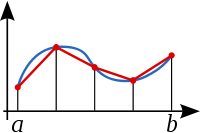
The trapezoid rule is a very simple method for estimating integrals. The idea is to approximate the area under a curve by a bunch of thin trapezoids and add up the areas of the trapezoids as suggested in the image below.

This is an old idea, probably older than the formal definition of an integral. In general it gives a crude estimation of the integral. If the width of the trapezoids is h, the error in using the trapezoid rule is roughly proportional to h². It’s easier to do better. For example, Simpson’s rule is a minor variation on the trapezoid rule that has error proportional to h⁵.

So if the trapezoid rule is old and inaccurate, why does anyone care about it? Here are the surprises.

You can still get a publication out of the trapezoid rule! In 1994, a doctor published a paper reinventing the trapezoid rule. Not only did the editors not recognize this ancient algorithm, the paper has been cited many times since it was published. (Update: more about the trapezoid paper here.)
Although the trapezoid rule is inefficient in general, it can be shockingly efficient for periodic functions.
The trapezoid rule can also be shockingly efficient for analytic functions that go to zero quickly, so called double exponential functions.

The last two observations are more widely applicable than you might think at first. What if you want to integrate something that isn’t periodic and isn’t a double exponential function? You may be able to do a change of variables that makes your integrand have one of these special forms. The article Fast Numerical Integration explains an integration method based on double exponential functions and includes C++ source code.

The potential efficiency of the trapezoid rule illustrates a general principle: a crude method cleverly applied can beat a clever technique crudely applied. The simplest numerical integration technique, one commonly taught in freshman calculus, can be extraordinarily efficient when applied with skill to the right problem. Conversely, a more sophisticated integration technique such as Gauss quadrature can fail miserably when naively applied.

Why IEEE floats have two zeros: +0 and −0

Posted on 15 June 2010 by John

Here’s a strange detail of IEEE floating point arithmetic: computers have two versions of 0: positive zero and negative zero. Most of the time the distinction between +0 and −0 doesn’t matter, but once in a while signed versions of zero come in handy.

If a positive quantity underflows to zero, it becomes +0. And if a negative quantity underflows to zero, it becomes −0. You could think of +0 (respectively, −0) as the bit pattern for a positive (negative) number too small to represent.

The IEEE floating point standard says 1/+0 should be +infinity and 1/−0 should be -infinity. This makes sense if you interpret ± 0 as the ghost of a number that underflowed leaving behind only its sign. The reciprocal of a positive (negative) number too small to represent is a positive (negative) number too large to represent.

To demonstrate this, run the following C code.

int main()
{
    double x = 1e-200;
    double y = 1e-200 * x;
    printf("Reciprocal of +0: %g\n", 1/y);
    y = -1e-200*x;
    printf("Reciprocal of -0: %g\n", 1/y);
}

On Linux with gcc the output is

Reciprocal of +0: inf
Reciprocal of -0: -inf

Windows with Visual C++ returns the same output except Windows prints infinity as 1#INF rather than inf. (See these notes for more on how Windows and Linux handle floating point exceptions.)

There is something, however, about signed zeros and exceptions that doesn’t make sense to me. The aptly named report “What Every Computer Scientist Should Know About Floating Point Arithmetic” has the following to say about signed zeros.

In IEEE arithmetic, it is natural to define log 0 = −∞ and log x to be a NaN when x < 0. Suppose that x represents a small negative number that has underflowed to zero. Thanks to signed zero, x will be negative, so log can return a NaN. However, if there were no signed zero, the log function could not distinguish an underflowed negative number from 0, and would therefore have to return −∞.

This implies log(-0) should be NaN and log(+0) should be -∞. That makes sense, but that’s not what happens in practice. The log function returns −∞ for both +0 and −0.

I ran the following code on Linux and Windows.

int main()
{
    double x = 1e-200;
    double y = 1e-200 * x;
    printf("Log of +0: %g\n", log(y));
    y = -1e-200*x;
    printf("Log of -0: %g\n", log(y));
}

On Linux, the code prints

Log of +0: -inf
Log of -0: -inf

The results were the same on Windows, except for the way Windows displays infinities.

Math library functions that seem unnecessary

Posted on 7 June 2010 by John

This post will give several examples of functions include in the standard C math library that seem unnecessary at first glance.

Function log1p(x) = log(1 + x)

The function log1p computes log(1 + x). How hard could this be to implement?

    log(1 + x);

Done.

But wait. What if x is very small? If x is 10⁻¹⁶, for example, then on a typical system 1 + x = 1 because machine precision does not contain enough significant bits to distinguish 1 + x from 1. (For details, see Anatomy of a floating point number.) That means that the code log(1 + x) would first compute 1 + x, obtain 1, then compute log(1), and return 0. But log(1 + 10⁻¹⁶) ≈ 10⁻¹⁶. This means the absolute error is about 10⁻¹⁶ and the relative error is 100%. For values of x larger than 10⁻¹⁶ but still fairly small, the code log(1 + x) may not be completely inaccurate, but the relative error may still be unacceptably large.

Fortunately, this is an easy problem to fix. For small x, log(1 + x) is approximately x. So for very small arguments, just return x. For larger arguments, compute log(1 + x) directly. See details here.

Why does this matter? The absolute error is small, even if the code returns a zero for a non-zero answer. Isn’t that OK? Well, it might be. It depends on what you do next. If you add the result to a large number, then the relative error in the answer doesn’t matter. But if you multiply the result by a large number, your large relative error becomes a large absolute error as well.

Function expm1(x) = exp(x) − 1

Another function that may seem unnecessary is expm1. This function computes e^x – 1. Why not just write this?

    exp(x) - 1.0;

That’s fine for moderately large x. For very small values of x, exp(x) is close to 1, maybe so close to 1 that it actually equals 1 to machine precision. In that case, the code exp(x) - 1 will return 0 and result in 100% relative error. As before, for slightly larger values of x the naive code will not be entirely inaccurate, but it may be less accurate than needed. The solution is to compute exp(x) − 1 directly without first computing exp(x). The Taylor series for exp(x) is 1 + x + x²/2 … So for very small x, we could just return x for exp(x) − 1. Or for slightly larger x, we could return x + x²/2. (See details here.)

Functions erf(x) and erfc(x)

The C math library contains a pair of functions erf and erfc. The “c” stands for “complement” because erfc(x) = 1 − erf(x). The function erf(x) is known as the error function and is not trivial to implement. But why have a separate routine for erfc? Isn’t it trivial to implement once you have code for erf? For some values of x, yes, this is true. But if x is large, erf(x) is near 1, and the code 1 - erf(x) may return 0 when the result should be small but positive. As in the examples above, the naive implementation results in a complete loss of precision for some values and a partial loss of precision for other values.

Functions Γ(x) and log Γ(x)

The standard C math library has two functions related to the gamma function: tgamma that returns Γ(x) and lgamma that return log Γ(x). Why have both? Why can’t the latter just use the log of the former? The gamma function grows extremely quickly. For moderately large arguments, its value exceeds the capacity of a computer number. Sometimes you need these astronomically large numbers as intermediate results. Maybe you need a moderate-sized number that is the ratio of two very large numbers. (See an example here.) In such cases, you need to subtract lgamma values rather than take the ratio of tgamma values. (Why is the function called “tgamma” and not just “gamma”? See the last paragraph and first comment on this post.)

Conclusion

The standard C math library distills a lot of experience. Some of the functions may seem unnecessary, and so they are for some arguments. But for other arguments these functions are indispensable.

What’s so hard about finding a hypotenuse?

Posted on 2 June 2010 by John

Numerical libraries usually have a function for finding the hypotenuse of a right triangle. Isn’t this trivial? If the sides of a triangle are x and y, just write this:

    sqrt(x*x + y*y)

That works in theory, but in practice it may fail. If x is so large that x*x overflows, the code will produce an infinite result.

We’d like to be able to say to the computer “Now x*x and y*y might be too big, but just wait a minute. I’m going to take a square root, and so the numbers will get smaller. I just need to borrow some extra range for a minute.” You can do something like that in environments that have extended precision, but that would be inefficient and unnecessary. And of course it would fail completely if you’re already using the largest numeric type available.

Here’s how to compute sqrt(x*x + y*y) without risking overflow.

max = maximum(|x|, |y|)
min = minimum(|x|, |y|)
r = min / max
return max*sqrt(1 + r*r)

Notice that the square root argument is between 1 and 2 and so there is no danger of overflow in taking the square root. The only way the algorithm could overflow is if the result itself is too large to represent. In that case the fault lies with the problem, not the algorithm: the algorithm was asked to compute a quantity larger than the largest representable number, and so it does the correct thing by overflowing and returning an infinite value. However, the algorithm will not unnecessarily return an infinite value due to an overflow in an intermediate computation.

To see how the algorithm above may succeed when the naive implementation would fail, let M be the largest representable number. For IEEE double precision, M is on the order of 10^308. All that matters for this example is that M is greater than 4. Let x and y equal 0.5 M. The algorithm above would return 0.707 M. But the naive algorithm would compute x*x and overflow since 0.25 M² > M. Then x*x + y*y would evaluate to infinity and the square root would evaluate to infinity.

A hypotenuse function is included in math.h on every system that I am aware of. It may be named hypot or _hypot.

Ten surprises from numerical linear algebra

Posted on 20 January 2010 by John

Here are ten things about numerical linear algebra that you may find surprising if you’re not familiar with the field.

Numerical linear algebra applies very advanced mathematics to solve problems that can be stated with high school mathematics.
Practical applications often require solving enormous systems of equations, millions or even billions of variables.
The heart of Google is an enormous linear algebra problem. PageRank is essentially an eigenvalue problem.
The efficiency of solving very large systems of equations has benefited at least as much from advances in algorithms as from Moore’s law.
Many practical problems — optimization, differential equations, signal processing, etc. — boil down to solving linear systems, even when the original problems are non-linear. Finite element software, for example, spends nearly all its time solving linear equations.
A system of a million equations can sometimes be solved on an ordinary PC in under a millisecond, depending on the structure of the equations.
Iterative methods, methods that in theory require an infinite number of steps to solve a problem, are often faster and more accurate than direct methods, methods that in theory produce an exact answer in a finite number of steps.
There are many theorems bounding the error in solutions produced on real computers. That is, the theorems don’t just bound the error from hypothetical calculations carried out in exact arithmetic but bound the error from arithmetic as carried out in floating point arithmetic on computer hardware.
It is hardly ever necessary to compute the inverse of a matrix.
There is remarkably mature software for numerical linear algebra. Brilliant people have worked on this software for many years.

More applied linear algebra

Don’t invert that matrix

Posted on 19 January 2010 by John

There is hardly ever a good reason to invert a matrix.

What do you do if you need to solve Ax = b where A is an n x n matrix? Isn’t the solution A⁻¹ b? Yes, theoretically. But that doesn’t mean you need to actually find A⁻¹. Solving the equation Ax = b is faster than finding A⁻¹. Books might write the problem as x = A⁻¹ b, but that doesn’t mean they expect you to calculate it that way.

What if you have to solve Ax = b for a lot of different b‘s? Surely then it’s worthwhile to find A⁻¹. No. The first time you solve Ax = b, you factor A and save that factorization. Then when you solve for the next b, the answer comes much faster. (Factorization takes O(n³) operations. But once the matrix is factored, solving Ax = b takes only O(n²) operations. Suppose n = 1,000. This says that once you’ve solved Ax = b for one b, the equation can be solved again for a new b 1,000 times faster than the first one. Buy one get one free.)

What if, against advice, you’ve computed A⁻¹. Now you might as well use it, right? No, you’re still better off solving Ax = b than multiplying by A⁻¹, even if the computation of A⁻¹ came for free. Solving the system is more numerically accurate than the performing the matrix multiplication.

It is common in applications to solve Ax = b even though there’s not enough memory to store A⁻¹. For example, suppose n = 1,000,000 for the matrix A but A has a special sparse structure — say it’s banded — so that all but a few million entries of A are zero. Then A can easily be stored in memory and Ax = b can be solved very quickly. But in general A⁻¹ would be dense. That is, nearly all of the 1,000,000,000,000 entries of the matrix would be non-zero. Storing A requires megabytes of memory, but storing A⁻¹ would require terabytes of memory.

Related post: Applied linear algebra

Numerical analysis