Computing arccos

Posted on 9 November 2022 by John

Suppose you take two numbers, a and b, and repeatedly take their arithmetic mean and their geometric mean. That is, suppose we set

a₀ = a
b₀ = b

then

a₁ = (a₀ + b₀)/2
b₁ = √(a₀ b₀)

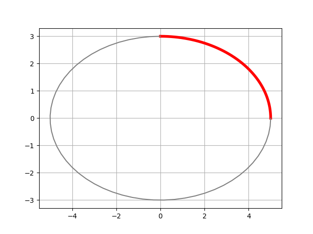
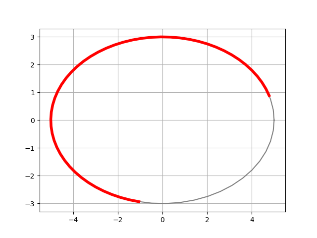
and repeat this process, each new a becoming the arithmetic mean of the previous a and b, and each new b becoming the geometric mean of the previous a and b. The sequence of a‘s and b‘s converge to a common limit, unsurprisingly called the arithmetic-geometric mean of a and b, written AGM(a, b).

Gauss found that AGM(a, b) could be expressed as an elliptic integral K:

AGM(a, b) = π(a + b) / 4K((a–b)/(a+b)).

You might read that as saying “OK, if I ever need to compute the AGM, I can do it by calling a function that evaluates K.” That’s true, but in practice it’s backward! The sequence defining the AGM converges very quickly, and so it is used to compute K.

Because the AGM converges so quickly, you may wonder what else you might be able to compute using a variation on the AGM. Gauss knew you could compute inverse cosine by altering the AGM. This idea was later rediscovered and developed more thoroughly by C. W. Borchardt and is now known as Borchardt’s algorithm. This algorithm iterates the following.

a₁ = (a₀ + b₀)/2
b₁ = √(a₁ b₀)

It’s a small, slightly asymmetric variant of the AGM. Instead of taking the geometric mean of the previous a and b, you take the geometric mean of the new a and the previous b.

I am certain someone writing a program to compute the AGM has implemented Borchardt’s algorithm by mistake. It’s what you get when you update a and b sequentially rather than simultaneously. But if you want to compute arccos, it’s a feature, not a bug.

Borchardt’s algorithm computes arccos(a/b) as √(b² – a²) divided by the limit of his iteration. Here it is in Python.

    def arccos(a, b):
       "Compute the inverse cosine of a/b."
        assert(0 <= a < b) 
        L = (b**2 - a**2)**0.5 
        while abs(a - b) > 1e-15:
            a = 0.5*(a + b)
            b = (a*b)**0.5
        return L/a

We can compare our implementation of inverse cosine with the one in NumPy.

    import numpy as np

    a, b = 2, 3
    print( arccos(a, b) )
    print( np.arccos(a/b) )

Both agree to 15 figures as we’d hope.

A small variation on the function above can compute inverse hyperbolic cosine.

    def arccosh(a, b):
        "Compute the inverse hyperbolic cosine of a/b."
        assert(a > b > 0)
        L = (a**2 - b**2)**0.5
        while abs(a - b) > 1e-15:
            a = 0.5*(a + b)
            b = (a*b)**0.5
        return L/a

Again we can compare our implementation to the one in NumPy

    a, b = 7, 4
    print( arccosh(a, b) )
    print( np.arccosh(a/b) )

and again they agree to 15 figures.

In an earlier post I wrote about Bille Carlson’s work on elliptic integrals, finding a more symmetric basis for these integrals. A consequence of his work, and possibly a motivation for his work, was to be able to extend Borchardt’s algorithm.” He said in [1]

The advantage of using explicitly symmetric functions is illustrated by generalizing Borchardt’s iterative algorithm for computing an inverse cosine to an algorithm for computing an inverse elliptic cosine.

I doubt Borchardt’s algorithm is used to compute arccos except in special situations. Maybe it’s used for extended precision. If you had an extended precision library without an arccos function built in, you could implement your own as above.

The practical value of Borschardt’s algorithm today is more likely in evaluating elliptic integrals. It also alludes to a deep theoretical connection between AGM-like iterations and elliptic-like integrals.

[1] B. C. Carlson. Hidden Symmetries of Special Function. SIAM Review , Jul., 1970, Vol. 12, No. 3 (Jul., 1970), pp. 332‐345

Carlson’s elliptic integrals

Posted on 7 November 2022 by John

Bille Carlson (1924-2013)

Although its a little fuzzy to say exactly which functions are “special” functions, these are generally functions that come up frequently in applications, that have numerous symmetries, and that satisfy many useful identities. The copious interconnections between special functions that are part of what makes them special also makes these functions hard to organize: everything is connected to everything else.

Bille Carlson did a great deal to simplify the study of special functions. With the benefit of decades of hindsight, Carlson discovered how several special functions should have been defined. I wrote a few weeks ago about how Carlson’s approach to Bessel functions eliminates unnecessary branch cuts. This post will look at how he simplified elliptic integrals.

The previous post looked at Legendre’s theorem showing that all elliptic integrals can be expressed in terms of three special functions—F, E, and Π— along with elementary functions. Carlson showed that Legendre’s three functions could be expressed in terms of two new functions. The advantage to Carlson’s approach is not that he reduced three functions down to two, but that his functions are symmetric. Hidden symmetries of elliptic integrals become obvious by definition.

Carlson’s elliptic functions

Carlson’s two basic functions are R_F and R_J defined below.

$\begin{align*} R_F(x,y,z) &= \tfrac{1}{2}\int_0^\infty \frac{dt}{\sqrt{(t+x)(t+y)(t+z)}} \\ R_J(x,y,z,p) &= \tfrac{3}{2}\int_0^\infty \frac{dt}{(t+p)\sqrt{(t+x)(t+y)(t+z)}} \end{align*}$

These functions are obviously symmetric in x, y, and z.

In addition, Carlson defined three more functions for convenience. The functions R_C and R_D are simple variations on R_F and R_J.

$\begin{align*} R_C(x,y) &= R_F(x, y, y) \\ R_D(x,y,z) &= R_J(x, y, z, z) \end{align*}$

Finally, his function R_G is defined by

$R_G(x,y,z) = \tfrac{1}{4}\int_0^\infty \frac{t\left(\frac{x}{t+x} + \frac{y}{t+y} + \frac{z}{t + z} \right)}{\sqrt{(t+x)(t+y)(t+z)}}\, dt$

The function R_G can be expressed in terms of R_F and R_D as follows, but the form above makes its symmetry obvious.

$2R_G(x, y, z) = z R_F(x, y, z) - \tfrac{1}{3} (x-z)(y-z) R_D(x, y, z) + \sqrt{\frac{xy}{z}}$

See [1].

Legendre to Carlson

Legendre’s elliptic integrals of the first, second, and third kinds can be related to Carlson’s symmetric functions as follows.

$\begin{align*} F(\phi,k) &=\sin\phi R_F\left(\cos^2\phi,1-k^2\sin^2\phi,1\right) \\ E(\phi,k) &=\sin\phi R_F\left(\cos^2\phi,1-k^2\sin^2\phi,1\right) \\ &\phantom{=}-\tfrac{1}{3}k^2\sin^3\phi R_D\left(\cos^2\phi,1-k^2\sin^2\phi,1\right) \\ \Pi(\phi,n,k) &=\sin\phi R_F\left(\cos^2\phi,1-k^2\sin^2\phi,1\right) \\ &\phantom{=}+\tfrac{1}{3}n\sin^3\phi R_J\left(\cos^2\phi,1-k^2\sin^2\phi,1,1-n\sin^2\phi\right) \end{align*}$

The correspondence between Legendre’s functions and Carlson’s functions is fairly complex. You could think of Carlson’s functions as a change of coordinates that makes things simpler, like describing the motion of planets from the perspective of the sun rather than the perspective of the earth.

The elliptic integrals discussed in this post have been the “incomplete” elliptic integrals. The identities for the corresponding complete elliptic integrals follow by setting φ = π/2.

$\begin{align*} K(k) &=R_F\left(0,1-k^2,1\right) \\ E(k) &=R_F\left(0,1-k^2,1\right)-\tfrac{1}{3}k^2 \,R_D\left(0,1-k^2,1\right) \\ \Pi(n,k) &=R_F\left(0,1-k^2,1\right)+\tfrac{1}{3}n \,R_J \left(0,1-k^2,1,1-n\right) \end{align*}$

Software support

In Python, scipy.special has functions ellipr* to implement each of Carlson’s R_* functions. That is, elliprc, elliprd, elliprf, elliprg, and elliprj implement R_C, R_D, R_F, R_G, and R_J respectively.

Similarly, Mathematica has functions CarlsonR*. That is, CarlsonRC, CarlsonRD, CarlsonRF, CarlsonRG, and CarlsonRJ implement R_C, R_D, R_F, R_G, and R_J respectively.

[1] B. C. Carlson. Numerical Computation of Real or Complex Elliptic Integrals. Available on arXiv.

Kinds of elliptic integrals

Posted on 7 November 2022 by John

Adrien-Marie Legendre caricature watercolor

There are three fundamental kinds of elliptic integrals, and these are prosaically but unhelpfully called elliptic integrals of the first kind, the second kind, and the third kind. These names sound odd to modern ears, but it’s no different than classical musicians naming symphonies Symphony No. 1, Symphony No. 2, etc.

This post covers the classical forms of elliptic integrals dating back to Adrien-Marie Legendre (1752–1833) and the next post will cover the modern formulation by Bille Carlson (1924–2013).

Comparing Legendre and Beethoven

This post will present Legendre’s classification theorem for elliptic integrals, but first let’s look at a few similarities between Legendre and Beethoven.

The image above is a caricature of Legendre, which is unfortunately the only image we have of him. But in this watercolor Legendre looks a little like Beethoven.

Legendre was studying elliptic integrals while Beethoven was writing symphonies—Legendre published his classification of elliptic integrals around a year after Beethoven finished his 9th symphony—and there was a common aesthetic in how they named things

A name like “Symphony No. 5 in C minor” isn’t that descriptive. If we know the difference between Beethoven’s Symphony No. 4 and Symphony No. 5, it’s because we’ve become familiar with each symphony; the names alone aren’t significant. It’s not as if Beethoven’s fourth symphony was written in 4/4 time and his fifth in 5/4 or anything like that.

But we just accept that that’s the way classical composers named things, and we should extend the same understanding to mathematics of the same era. Legendre named his functions analogously to the way Beethoven named his symphonies.

Elliptic integrals

Before we classify elliptic integrals, we should say what elliptic integrals are. These are functions of the form

$f(x) = \int_0^x R(t, \sqrt{P(t)}) \, dt$

where R is a rational function and P is a polynomial of degree three or four.

Classification

Legendre’s classification theorem says that any elliptic integral can be written as a linear combination of elementary functions and three special functions: F, E, and Π. These are the elliptic integrals of the first, second, and third kind, defined below. Said another way, you can evaluate elliiptic integrals if you add just three advanced functions—F, E, and Π— to the set of functions covered in a calculus class.

The elliptic integral of the second kind comes up in calculating the length of an elliptic arc, and the family of elliptic integrals take their name from this association. I think of E as mnemonic for “ellipse” and F as mnemonic for “first.” I don’t know whether this was the original motivation for the names. Legendre was French, and I doubt he would call a function F for “first” because the French word for “first” is première. Maybe an English speaker came up with the notation.

Elliptic integrals of the first kind describe the motion of a pendulum [1]. So you might think of F as pendulum functions. It would have been nice if these functions were denoted P rather than F; French speakers could think P stands for “première” and English speakers could think it stand for “pendulum.”

At least in my experience, elliptic integrals of the second kind come up most often, with elliptic integrals of the first kind a distant second, and elliptic integrals of the third kind are rare. I believe my experience is typical; many sources only discuss integrals of the first and second kind and leave out integrals of the third kind.

Definitions

Here are Legendre’s three basic elliptic integrals.

$\begin{align*} F(\varphi; k) &= \int_0^\varphi \frac{d\theta}{\sqrt{1 - k^2 \sin^2\theta}} \\ E(\varphi; k) &= \int_0^\varphi \sqrt{1 - k^2 \sin^2\theta} \, d\theta \\ \Pi(n; \varphi, k) &= \int_0^\varphi \frac{d\theta}{(1 - n\sin^2\theta)\sqrt{1 - k^2 \sin^2\theta}} \\ \end{align*}$

Elliptic integrals versus elliptic functions

Elliptic integrals are functions defined by integrals. They’re not the same as elliptic functions, though there’s a connection. It is often said that the inverse of an elliptic integral is an elliptic function. That’s not true without some qualification. What’s true is that the inverse of an elliptic integral of the first kind is an elliptic function.

[1] The equation for pendulum motion that is first introduced to students makes the simplifying assumption that the displacement angle θ is so small that sin θ can be replaced with θ. In this case the motion is described by sines and cosines. But if you don’t make this assumption, then the differential equation for motion is nonlinear and its solution is an elliptic integral of the first kind.

How to calculate length of an elliptic arc

Posted on 2 November 2022 by John

This post will show how to find the length of piece of an ellipse and explain what elliptic integrals have to do with ellipses.

Assume we have an ellipse centered at the origin with semi-major axis a and semi-minor axis b. So a > b > 0, the longest diameter of the ellipse is 2a and the shortest is 2b. The ellipse can be parameterized by

$\begin{align*} x(t) &= a \cos(t) \\ y(t) &= b \sin(t) \end{align*}$

Special case: quarter of an ellipse

Let’s first find the perimeter of a 1/4 of the ellipse.

one quarter of an ellipse highlighted in red

This is given by the integral

$\int_0^{\pi/2} \sqrt{a^2 \sin^2(t) + b^2 \cos^2(t)}\, dt$

The change of variables u = π/2 – t turns the integral into

$\begin{align*} \int_0^{\pi/2} \sqrt{a^2 \cos^2(u) + b^2 \sin^2(u)}\, du &= a \int_0^{\pi/2} \sqrt{1 - \left(1 - b^2/a^2 \right) \sin^2(u)}\, du \\ &= a E\left(1 - b^2/a^2 \right) \end{align}$

because E, the “elliptic integral of the second kind,” is defined by

$E(m) = \int_0^{\pi/2} \sqrt{1 - m\sin^2 t}\, dt$

Therefore the perimeter of the entire ellipse is 4aE(1 – b²/a²). Let’s define

for the rest of the post. Incidentally, m = e² where e is the eccentricity of the ellipse.

General case

Now let’s find the length of an arc where t ranges from 0 to T and T is not necessarily π/2.

general elliptic segment highlighted in red

The derivation is similar to that above.

$\begin{align*} \int_0^T \sqrt{a^2\sin^2(t) + b^2\cos^2(t)}\, dt &= \int_{\pi/2 - T}^{\pi/2} \sqrt{a^2\cos^2u + b^2\sin^2u} \, du \\ &= a E(m) - a \int_0^{\pi/2 - T} \sqrt{1 - m \sin^2u} \, du \\ &= aE(m) -aE(\pi/2 - T, m) \\ &= a E(m) + a E(T - \pi/2, m) \end{align*}$

where E, now with two arguments, is the “incomplete elliptic integral of the second kind” defined by

$E(\varphi, m) = \int_0^\varphi \sqrt{1 - m\sin^2(t)} \,dt$

It is “incomplete” because we haven’t completed the integral by integrating all the way up to π/2.

To find the length of a general arc whose parameterization runs from t = T₀ to t = T₁ we find the length from 0 out to T₁ and subtract the length from 0 out to T₀ which gives us

$a E(T_1 - \pi/2, m) - a E(T_0 - \pi/2, m)$

The elliptic integrals are so named because they came out of the problem we’re looking at in this post. The integrals cannot be computed in elementary terms, so we introduce new functions that are defined by the integrals. I expand this idea in this post.

NB: We are specifying arcs by the range of our parameterization parameter t, not by the angle from the center of the ellipse. If our ellipse were a circle the two notions would be the same, but in general they are not. The central angle θ and the parameter T are related via

$\begin{align*} \theta &= \arctan\left( \frac{b}{a} \tan T \right) \\ T &= \arctan\left( \frac{a}{b} \tan\theta \right) \end{align*}$

I wrote about this here.

Python code

Let’s calculate the length of an arc two ways: using our formula and using numerical integration. Note that the Python implementation of the (complete) elliptic integral is ellipe and the implementation of the incomplete elliptic integral is ellipeinc. The “e” at the end of ellipe distinguishes this elliptic integral, commonly denoted by E, from other kinds of elliptic integrals.

    
    from numpy import pi, sin, cos
    from scipy.special import ellipe, ellipeinc
    from scipy.integrate import quad
    
    def arclength(T0, T1, a, b):
        m = 1 - (b/a)**2
        t1 = ellipeinc(T1 - 0.5*pi, m)
        t0 = ellipeinc(T0 - 0.5*pi, m)
        return a*(t1 - t0)
    
    def numerical_length(T0, T1, a, b):
        f = lambda t: (a**2*sin(t)**2 + b**2*cos(t)**2)**0.5
        return quad(f, T0, T1)
        
    T0, T1, a, b = 0, 1, 3, 2
    y, err = numerical_length(T0, T1, a, b)
    ell = arclength(T0, T1, a, b)
    assert(abs(ell - y) < 1e-12)

    T0, T1, a, b = 7, 1, 4, 3
    y, err = numerical_length(T0, T1, a, b)
    ell = arclength(T0, T1, a, b)
    assert(abs(ell - y) < 1e-12)

The tests pass. This increases our confidence that the derivation above is correct.

Eliminating a Bessel function branch cut

Posted on 6 September 2022 by John

In an earlier post I looked in detail at a series for inverse cosine centered at 1. The function arccos(z) is multivalued in a neighborhood of 1, but the function

arccos(z) / √(2 – 2z)

is analytic in a neighborhood of 1. We cancel out the bad behavior of inverse cosine at 1 by dividing by another function with matching bad behavior.

We can do something similar with Bessel functions. In general, the Bessel function J_ν has a branch cut from -∞ to 0. But the function

J_ν / z^ν

is entire, i.e. analytic everywhere in the complex plane. From a certain perspective—namely the perspective advocated by Bille Carlson (1924–2013)—we got the definition of Bessel functions (and other functions) wrong. Carlson’s book Special Functions of Applied Mathematics shows how many special functions can be defined in terms of a smaller number of functions with fewer branch cuts. This simplification revealed symmetries that hadn’t been noticed before.

Here’s a plot of J_1/3(z). Height represents magnitude and color represents phase.

This was produced using the Mathematica command

    ComplexPlot3D[BesselJ[1/3, z], {z, -1 - I, 1 + I}]

The abrupt change from purple to yellow along the negative real axis shows the discontinuity in the phase at the branch cut. You can also see a hint of the cusp at the origin.

Here’s a plot of J_1/3(z) / z^1/3.

This was made using

    ComplexPlot3D[BesselJ[1/3, z]/z^(1/3), {z, -1 - I, 1 + I}]

The white streak is an artifact of the branch cuts for J_1/3(z) and for z^1/3. The branch cut in their ratio is unnecessary.

Numerically evaluating a theta function

Posted on 22 June 2022 by John

Theta functions pop up throughout pure and applied mathematics. For example, they’re common in analytic number theory, and they’re solutions to the heat equation.

Theta functions are analogous in some ways to trigonometric functions, and like trigonometric functions they satisfy a lot of identities. This post will comment briefly on an identity that makes a particular theta function, θ₃, easy to compute numerically. And because there are identities relating the various theta functions, a method for computing θ₃ can be used to compute other theta functions.

The function θ₃ is defined by

$\theta_3(z, t) = 1 + \sum_{k=1}^\infty q^{k^2} \cos(2kz)$

where

$q = e^{\pi i t}$

Here’s a plot of θ₃ with t = 1 + i

produced by the following Mathematica code:

    
    q = Exp[Pi I (1 + I)]
    ComplexPlot3D[EllipticTheta[3, z, q], {z, -1, 8.5 + 4 I}]

An important theorem tells us

$\theta_3(z, t) = (-it)^{-1/2} \exp(z^2/\pi i t)\, \theta_3\left(\frac{z}{t}, -\frac{1}{t} \right )$

This theorem has a lot of interesting consequences, but for our purposes note that the identity has the form

$\theta_3(\ldots, t) = \ldots \theta_3\left(\ldots, -\frac{1}{t} \right )$

The important thing for numerical purposes is that t is on one side and 1/t is on the other.

Suppose t = a + bi with a > 0 and b > 0. Then

$q = \exp\left(\pi i (a + bi)\right) = \exp(-\pi b) \exp(\pi i a)$

Now if b is small, |q| is near 1, and the series defining θ₃ converges slowly. But if b is large, |q| is very small, and the series converges rapidly.

So if b is large, use the left side of the theorem above to compute the right. But if b is small, use the right side to compute the left.

Architecture and Math

Posted on 1 January 2022 by John

I recently received a review copy of Andrew Witt’s new book Formulations: Architecture, Mathematics, and Culture.

The Hankel function on the cover is the first clue that this book contains some advanced mathematics. Or rather, it references some advanced mathematics. I’ve only skimmed the book so far, but I didn’t see any equations.

Hankel functions are defined in terms of Bessel functions:

$H^{(1)}_\nu(z) = J_\nu(z) + i Y_\nu(z)$

where J is the Bessel function of the first kind, Y is the Bessel function of the second kind, and ν is the order. I’ve only ever seen one subscript on Hankel functions, but my suspicion is that the two subscripts allow for different orders on J and Y. That is, my guess is that

$H^{(1)}_{(m,n)}(z) = J_m(z) + i Y_n(z)$

Here’s my quick attempt to reproduce the cover art in Mathematica:

    H[m_, n_, z_] := BesselJ[m, z] + I BesselY[n, z]
    ComplexPlot3D[H[3, 5, z], {z, -4 - 4 I, 5 + 5 I}]

This produces the following plot.

I’m amazed that people ever had the patience and skill to manually make plots like the one on the cover of Witt’s book.

While thumbing through the book I noticed some curves that I recognized as Lissajous curves. Turns out these were curves made by Lissajous himself. The plots were accompanied by the mechanical devices Lissajous used to draw them.

The exception case is normal

Posted on 27 December 2021 by John

Sine and cosine have power series with simple coefficients, but tangent does not. Students are shocked when they see the power series for tangent because there is no simple expression for the power series coefficients unless you introduce Bernoulli numbers, and there’s no simple expression for Bernoulli numbers.

The perception is that sine and cosine are the usual case, and that tangent is exceptional. That’s because in homework problems and examples, sine and cosine are the usual case, and tangent is exceptional. But as is often the case, the pedagogically convenient case is the exception rather than the rule.

Of the six common trig functions—sine, cosine, tangent, secant, cosecant, cotangent—sine and cosine are the only ones with power series not involving Bernoulli numbers. The power series for most of the common trig functions require Bernoulli numbers.

Details

The functions cosecant and cotangent have a singularity at 0, so the power series for these functions at 0 are Laurant series rather than Taylor series, i.e. they involve negative as well as positive exponents. We will look at z csc(z) and z cot(z) because multiplying by z removes the singularity.

$\begin{align*} \sin(z) &= \sum_{n=0}^\infty (-1)^n \frac{ z^{2n+1} }{ (2n+1)! } \\ \cos(z) &= \sum_{n=0}^\infty (-1)^n \frac{ z^{2n} }{ (2n)! } \\ \tan(z) &= \sum_{n=1}^\infty (-1)^{n-1} 4^n (4^n-1) B_{2n} \frac{ z^{2n-1} }{ (2n)! } \\ \text{sec}(z) &= \sum_{n=0}^\infty (-1)^n E_{2n} \frac{ z^{2n} }{ (2n)! } \\ z\text{cot}(z) &= \sum_{n=0}^\infty (-4)^n B_{2n} \frac{ z^{2n} }{ (2n)! } \\ z\text{csc}(z) &= \sum_{n=0}^\infty (-1)^{n-1} (2^{2n} - 2) B_{2n} \frac{ z^{2n} }{ (2n)! } \end{align*}$

The series for secant doesn’t use Bernoulli numbers directly but rather Euler numbers. However, Bernoulli and Euler numbers are closely related.

$\begin{align*} B_n &= \sum_{k=0}^{n-1} \binom{n-1}{k} \frac{n}{4^n - 2^n} E_k \\ E_n &= \sum_{k=1}^{n} \binom{n}{k-1} \frac{2^n - 4^n}{k} B_k \end{align*}$

The zeta distribution

Posted on 10 December 2021 by John

The previous post on the Yule-Simon distribution mentioned the zeta distribution at the end. This is a powerlaw distribution on the positive integers with normalizing constant given by the Riemann zeta distribution. That is, the zeta distribution has density

f(k; s) = k^–s / ζ(s).

where k is a positive integer and s > 1 is a fixed parameter.

For s > 1, the zeta function is defined as the sum of the positive integers to the power negative s, so ζ(s) is essentially defined as the normalizing constant of the zeta distribution.

I wanted to make a couple comments about this. First, it shows that the zeta function appears in applications outside of number theory. Second, when working with the zeta distribution, it would be useful to have an estimate for ζ(s).

Zeta function bounds

The integral test in calculus is typically presented as a way to test whether an infinite sum converges. This is a shame. In analysis as in statistics, estimation is better than testing. Testing throws away continuous information and replaces it with a single bit.

Let f(x) be a decreasing function; we have in mind f(x) = 1/x^s. Then for any n,

$\int_{n+1}^\infty f(x)\, dx \leq \sum_{k = n+1}^\infty f(k) \leq \int_{n}^\infty f(x)\, dx$

To estimate a sum over k, we sum the first n terms directly and apply the inequalities above for the rest. Typically n will be small, maybe 0 or 1. A larger value of n will give more accurate bounds but at the expense of a more complicated expression.

When f(x) = 1/x^s and n is at least 1, we have

$\frac{(n+1)^{1-s}}{s-1} \leq \sum_{k = n+1}^\infty f(k) \leq \frac{n^{1-s}}{s-1}$

This says

$\sum_{k=1}^n k^{-s} + \frac{(n+1)^{1-s}}{s-1} \leq \zeta(s) \leq \sum_{k=1}^n k^{-s} + \frac{n^{1-s}}{s-1}$

This gives a good lower bound but a bad upper bound when we choose n = 1.

But it gives a much better upper bound when we choose n = 2.

3D Go with identities

Posted on 1 December 2021 by John

Let’s play a game that’s something like Go in three dimensions. Our game is played on the lattice of points in 3D that have integer coordinates. Someone places stones on two lattice points, and your job is to create a path connecting the two stones by adding stones to neighboring locations.

Game cube

We don’t really have a game “board” since we’re working in three dimensions. We have a game scaffold or game cube. And we can’t just put our stones down. We have to imagine the stones has having hooks that we can use to hang them where pieces of scaffolding come together.

Basic moves

Now for the rules. Our game is based on identities for a function with depending on three parameters: a, b, and c. A location in our game cube is a point with integer coordinates (i, j, k) corresponding to function parameters

(a+i, b+j, c+k).

If there is a stone at (i, j, k) then we are allowed to place stones at neighboring locations if there is a function identity corresponding to these points. The function identities are the “contiguous relations” for hypergeometric functions. You don’t need to know anything about hypergeometric functions to play this game. We’re going to leave out a lot of detail.

Our rule book for identities will be Handbook of Mathematical Function by Abramowitz and Stegun, widely known as A&S. You can find a copy online here.

For example, equation 15.2.10 from A&S relates

F(a, b; c; z)

F(a-1, b; c; z)

and

F(a+1, b; c; z).

So if we have a stone at (i, j, k) we can add stones at (i-1, j, k) and (i+1, j, k). Or we could add stones at (i+1, j, k) and (i+2, j, k). You can turn one stone into a row of three stones along the first axis overlapping the original stone.

Equation 15.2.11 lets you do something analogous for incrementing the 2nd coordinate, and Equation 15.2.12 lets you increment the 3rd coordinate. So you could replace a stone with a row of three stones along the second or third axes as well.

This shows that it is always possible to create a path between two lattice points. If you can hop between stones a distance 1 apart, you can create a path that will let you hop between any two points.

Advanced moves

There are other possible steps. For example, equation 15.2.25 has the form

… F(a, b; c; z) + … F(a, b-1; c; z) + … F(a, b; c+1; z) = 0

I’ve left out the coefficients above, denoting them by ellipses. (More on that below.) This identity says you don’t just have to place stones parallel to an axis. For example, you can add a stone one step south and another one step vertically in the same move.

The previous section showed that it’s always possible to create a path between two lattice points. This section implies the finding the shortest path between two points might be a little more interesting.

Applications

There are practical applications to the game described in this post. One reason hypergeometric functions are so useful is that they satisfy a huge number of identities. There are libraries of hypergeometric identities, and there are still new identities to discover and new patterns to discover for organizing the identities.

The moves in the game above can be used to speed up software. Hypergeometric functions are expensive to evaluate, and so it saves time to compute a new function in terms of previously computed functions rather than having to compute it from scratch.

I used this trick to speed up clinical trial simulations. Consecutive steps in the simulation required evaluating contiguous hypergeometric functions, so I could compute one or two expensive functions at the beginning of the simulation and bootstrap them to get the rest of the values I needed.

Coefficients

I’d like to close by saying something about the coefficients in these identities. The coefficients are complicated and don’t have obvious patterns, and so they distract from the underlying structure discussed here. You could stare at a list of identities for a while before realizing that apart from the coefficients the underlying relationships are simple.

All the coefficients in the identities cited above are polynomials in the variables a, b, c, and z. All have degree at most 2, and so they can be computed quickly.

The identities discussed here are often called linear relations. The relations are linear in the hypergeometric functions, but the coefficients are not linear.

Special functions

Computing arccos

Related posts

Carlson’s elliptic integrals

Carlson’s elliptic functions

Legendre to Carlson

Software support

Related posts

Kinds of elliptic integrals

Comparing Legendre and Beethoven

Elliptic integrals

Classification

Definitions

Elliptic integrals versus elliptic functions

Related posts

How to calculate length of an elliptic arc

Special case: quarter of an ellipse

General case

Python code

Eliminating a Bessel function branch cut

Related posts

Numerically evaluating a theta function

Related posts

Architecture and Math

Related posts

The exception case is normal

Details

Related posts

The zeta distribution

Zeta function bounds

Related posts

3D Go with identities

Game cube

Basic moves

Advanced moves

Applications

Coefficients

Related posts