The traditional approach to teaching differential equations is to present a collection of techniques for finding closed-form solutions to ordinary differential equations (ODEs). These techniques seem completely unrelated [1] and have arcane names such as integrating factors, exact equations, variation of parameters, etc.
Students may reasonably come away from an introductory course with the false impression that it is common for ODEs to have closed-form solutions because it is common in the class.
My education reacted against this. We were told from the beginning that differential equations rarely have closed-form solutions and that therefore we wouldn’t waste time learning how to find such solutions. I didn’t learn the classical solution techniques until years later when I taught an ODE class as a postdoc.
I also came away with a false impression, the idea that differential equations almost never have closed-form solutions in practice, especially nonlinear equations, and above all partial differential equations (PDEs). This isn’t far from the truth, but it is an exaggeration.
I specialized in nonlinear PDEs in grad school, and I don’t recall ever seeing a closed-form solution. I heard rumors of a nonlinear PDE with a closed form solution, the KdV equation, but I saw this as the exception that proves the rule. It was the only nonlinear PDE of practical importance with a closed-form solution, or so I thought.
It is unusual for a nonlinear PDE to have a closed-form solution, but it is not unheard of. There are numerous examples of nonlinear PDEs, equations with important physical applications, that have closed-form solutions.
Yesterday I received a review copy of Analytical Methods for Solving Nonlinear Partial Differential Equations by Daniel Arrigo. If I had run across with a book by that title as a grad student, it would have sounded as eldritch as a book on the biology of Bigfoot or the geography of Atlantis.
A few pages into the book there are nine exercises asking the reader to verify closed-form solutions to nonlinear PDEs:
- a nonlinear diffusion equation
- Fisher’s equation
- Fitzhugh-Nagumo equation
- Berger’s equation
- Liouville’s equation
- Sine-Gordon equation
- Korteweg–De Vries (KdV) equation
- modified Korteweg–De Vries (mKdV) equation
- Boussinesq’s equation
These are not artificial examples crafted to have closed-form solutions. These are differential equations that were formulated to model physical phenomena such as groundwater flow, nerve impulse transmission, and acoustics.
It remains true that differential equations, and especially nonlinear PDEs, typically must be solved numerically in applications. But the number of nonlinear PDEs with closed-form solutions is not insignificant.
Related posts
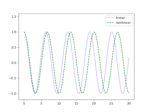
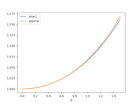
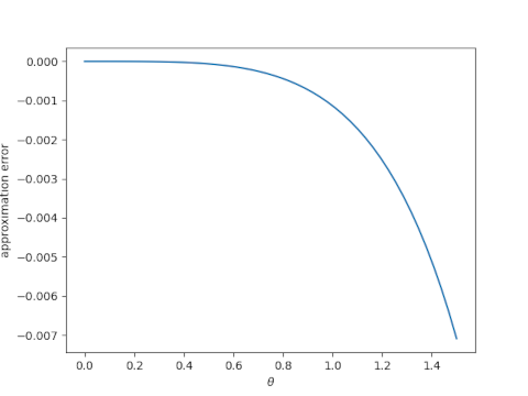
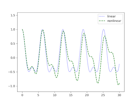
- Period of a nonlinear pendulum
- Rational solutions to KdV
- Trading generalized derivatives for classical ones
[1] These techniques are not as haphazard as they seem. At a deeper level, they’re all about exploiting various forms of symmetry.