Keeping data and code together with org-mode

With org-mode you can keep data, code, and documentation in one file.

Suppose you have an org-mode file containing the following table.

    #+NAME: mydata
    | Drug | Patients |
    |------+----------|
    |    X |      232 |
    |    Y |      351 |
    |    Z |      117 |

Note that there cannot be a blank line between the NAME header and the beginning of the table.

You can bring this table into Python simply by declaring it to be a variable in the header of a Python code block.

    #+begin_src python :var tbl=mydata :results output
    print(tbl)
    #+end_src

When you evaluate this block, you see that the table is imported as a list of lists.

    [['X', 232], ['Y', 351], ['Z', 117]]

Note that the column headings were not imported into Python. Now suppose you would like to retain the headers, and use them as column names in a pandas data frame.

    #+begin_src python :var tbl=mydata :colnames no :results output
    import pandas as pd
    df = pd.DataFrame(tbl[1:], columns=tbl[0])
    print(df, "\n")
    print(df["Patients"].mean())
    #+end_src

When evaluated, this block produces the following.

      Drug  Patients 
    0    X       232
    1    Y       351
    2    Z       117

    233.33333333333334

Note that in order to import the column names, we told org-mode that there are no column names! We did this with the header option

    :colnames no

This seems backward, but it makes sense. It says do bring in the first row of the table, even though it appears to be a column header that isn’t imported by default. But then we tell pandas that we want to make a data frame out of all but the first row (i.e. tbl[1:]) and we want to use the first row (i.e. tbl[0]) as the column names.

A possible disadvantage to keeping data and code together is that the data could be large. But since org files are naturally in outline mode, you could collapse the part of the outline containing the data so that you don’t have to look at it unless you need to.

Related posts

Haskell analog of Sweave and Pweave

Sweave and Pweave are programs that let you embed R and Python code respectively into LaTeX files. You can display the source code, the result of running the code, or both.

lhs2TeX is roughly the Haskell analog of Sweave and Pweave.  This post takes the sample code I wrote for Sweave and Pweave before and gives a lhs2TeX counterpart.

\documentclass{article}
%include polycode.fmt
%options ghci
\long\def\ignore#1{}
\begin{document}

Invisible code that sets the value of the variable $a$.

\ignore{
\begin{code}
a = 3.14
\end{code}
}

Visible code that sets $b$ and squares it. 

(There doesn't seem to be a way to display the result of a block of code directly. 
Seems you have to save the result and display it explicitly in an eval statement.)

\begin{code}
b = 3.15
c = b*b
\end{code}

$b^2$ = \eval{c}

Calling Haskell inline: $\sqrt{2} = \eval{sqrt 2}$

Recalling the variable $a$ set above: $a$ = \eval{a}.

\end{document}

If you save this code to a file foo.lhs, you can run

lhs2TeX -o foo.tex foo.lhs

to create a LaTeX file foo.tex which you could then compile with pdflatex.

One gotcha that I ran into is that your .lhs file must contain at least one code block, though the code block may be empty. You cannot just have code in \eval statements.

Unlike R and Python, the Haskell language itself has a notion of literate programming. Haskell specifies a format for literate comments. lhs2TeX is a popular tool for processing literate Haskell files but not the only one.

Basics of Sweave and Pweave

Sweave is a tool for embedding R code in a LaTeX file. Pweave is an analogous tool for Python. By putting your code in your document rather than the results of running your code somewhere else, results are automatically recomputed when inputs change. This is especially useful with graphs: rather than including an image into your document, you include the code to create the image.

To use either Sweave or Pweave, you create a LaTeX file and include source code inside. A code block begins with <<>>= and ends with @ on a line by itself. By default, code blocks appear in the LaTeX output. You can start a code block with <<echo=FALSE>>= to execute code without echoing its source. In Pweave you can also use <% and %> to mark a code block that executes but does not echo. You might want to do this at the top of a file, for example, for import statements.

Sweave echos code like the R command line, with > for the command prompt. Pweave does not display the Python >>> command line prompt by default, though it will if you use the option term=TRUE in the start of your code block.

In Sweave, you can use Sexpr to inline a little bit of R code. For example, $x = Sexpr{sqrt(2)}$ will produce x = 1.414…. You can also use Sexpr to reference variables defined in previous code blocks. The Pweave analog uses <%= and %>. The previous example would be $x = <%= sqrt(2) %>$.

You can include a figure in Sweave or Pweave by beginning a code block with <<fig=TRUE, echo=FALSE>>= or with echo=TRUE if you want to display the code that produces the figure. With Sweave you don’t need to do anything else with your file. With Pweave you need to add usepackage{graphicx} at the top.

To process an Sweave file foo.Rnw, run Sweave("foo.Rnw") from the R command prompt. To process a Pweave file foo.Pnw, run Pweave -f tex foo.Pnw from the shell. Either way you get a LaTeX file that you can then compile to a PDF.

Here are sample Sweave and Pweave files. First Sweave:

\documentclass{article}
\begin{document}

Invisible code that sets the value of the variable $a$.

<<<echo=FALSE>>=
a <- 3.14
@

Visible code that sets $b$ and squares it.

<<bear, echo=TRUE>>=
b <- 3.15
b*b
@

Calling R inline: $\sqrt{2} = Sexpr{sqrt(2)}$

Recalling the variable $a$ set above: $a = Sexpr{a}$.

Here's a figure:

<<fig=TRUE, echo=FALSE>>=
x <- seq(0, 6*pi, length=200)
plot(x, sin(x))
@

\end{document}

And now Pweave:

\documentclass{article}
\usepackage{graphicx}
\begin{document}

<%
import matplotlib.pyplot as plt
from numpy import pi, linspace, sqrt, sin
%>

Invisible code that sets the value of the variable $a$.

<<echo=FALSE>>=
a = 3.14
@

Visible code that sets $b$ and squares it.

<<term=True>>=
b = 3.15
print b*b
@

Calling Python inline: $\sqrt{2} = <%= sqrt(2) %>$

Recalling the variable $a$ set above: $a = <%= a %>$.

Here's a figure:

<<fig=True, echo=False>>=
x = linspace(0, 6*pi, 200)
plt.plot(x, sin(x))
plt.show()
@

\end{document}

Related links

Running Python and R inside Emacs

Emacs org-mode lets you manage blocks of source code inside a text file. You can execute these blocks and have the output display in your text file. Or you could export the file, say to HTML or PDF, and show the code and/or the results of executing the code.

Here I’ll show some of the most basic possibilities. For much more information, see  orgmode.org. And for the use of org-mode in research, see A Multi-Language Computing Environment for Literate Programming and Reproducible Research.

Source code blocks go between lines of the form

    #+begin_src
    #+end_src

On the #+begin_src line, specify the programming language. Here I’ll demonstrate Python and R, but org-mode currently supports C++, Java, Perl, etc. for a total of 35 languages.

Suppose we want to compute √42 using R.

    #+begin_src R
    sqrt(42)
    #+end_src

If we put the cursor somewhere in the code block and type C-c C-c, org-mode will add these lines:

    #+results:
    : 6.48074069840786

Now suppose we do the same with Python:

    #+begin_src python
    from math import sqrt
    sqrt(42)
    #+end_src

This time we get disappointing results:

    #+results:
    : None

What happened? The org-mode manual explains:

… code should be written as if it were the body of such a function. In particular, note that Python does not automatically return a value from a function unless a return statement is present, and so a ‘return’ statement will usually be required in Python.

If we change sqrt(42) to return sqrt(42) then we get the same result that we got when using R.

By default, evaluating a block of code returns a single result. If you want to see the output as if you were interactively using Python from the REPL, you can add :results output :session following the language name.

    #+begin_src python :results output :session
    print "There are %d hours in a week." % (7*24)
    2**10
    #+end_src

This produces the lines

    #+results:
    : There are 168 hours in a week.
    : 1024

Without the :session tag, the second line would not appear because there was no print statement.

I had to do a couple things before I could get the examples above to work. First, I had to upgrade org-mode. The version of org-mode that shipped with Emacs 23.3 was quite out of date. Second, the only language you can run by default is Emacs Lisp. You have to turn on support for other languages in your .emacs file. Here’s the code to turn on support for Python and R.

    (org-babel-do-load-languages
        'org-babel-load-languages '((python . t) (R . t)))

Update: My next post shows how to call code in written in one language from code written in another language.

Related posts

Readability

The Readability bookmarklet lets you reformat any web to make it easier to read. It strips out flashing ads and other distractions. It uses black text on a white background, wide margins, a moderate-sized font, etc. I use Readability fairly often. (Instapaper is a similar service. I discuss it at the end of this post.)

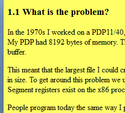
Yesterday I used it to reformat an article on literate programming. For some inexplicable reason, the author chose to use a lemon yellow background. It’s ironic that the article is about making source code easier to read. The content of the article is easy to read, but the format is not.

Readability to the rescue! Here are before and after screen shots.

Before:

After:

I recommend the article, Example of Literate Programming in HTML [Update: link went away], and I also recommend using reformatting the page unless you enjoy reading black text on a yellow background.

Readability did a good job until about half way through the article. The article has C and HTML code examples, and perhaps these confused Readability. (Readability usually handles code samples well. It correctly formats the first few code samples in this article.) The last half of the article renders like source code, and the font gets smaller and smaller.

I ran the page through an HTML validator to see whether some malformed HTML could be the source of the problem. The validator found numerous problems, so perhaps that was the issue.

I haven’t seen Readability fail like this before. I’ve been surprised how well it has handled some pages I thought might trip it up.

I ended up saving the article and editing its source, changing the bgcolor value to white. It’s a nice article on literate programming once you get past the formatting. The best part of the article is the first section, and that much Readability formats correctly.

Instapaper

Instapaper reformats web pages similarly. It produces a narrower column of text, but otherwise the output looks quite similar.

Instapaper did not discover the title of the literate programming article. (The title of the article was not in an <h1> tag as software might expect but was only in a <title> tag in the page header.) However, it did format the entire body of the article correctly.

I find it slightly more convenient to use the Readability bookmarklet than to submit a link to Instapaper. I imagine there are browser plug-ins that make Instapaper just as easy to use, though I haven’t looked into this because I’m usually satisfied with Readability.

Related posts

Computing the inverse of the normal CDF

Someone asked me this week for C++ code to compute the inverse of the normal (Gaussian) distribution function. The code I usually use isn’t convenient to give away because it’s part of a large library, so I wrote a stand-alone function using an approximation out of Abramowitz and Stegun (A&S). There are a couple things A&S takes for granted, so I decided to write up the code in the spirit of a literate program to explain the details. The code is compact and portable. It isn’t as fast as possible nor as accurate as possible, but it’s good enough for many purposes.

A literate program to compute the inverse of the normal CDF

Literate programming and statistics

Sweave, mentioned in my previous post, is a tool for literate programming. Donald Knuth invented literate programming and gives this description of the technique in his book by the same name:

I believe that the time is ripe for significantly better documentation of programs, and that we can best achieve this by considering programs to be works of literature. Hence, my title: “Literate Programming.”

Let us change our traditional attitude to the construction of programs: Instead of imagining that our main task is to instruct a computer what to do, let us concentrate rather on explaining to human beings what we want a computer to do.

The practitioner of literate programming can be regarded as an essayist, whose main concern is with exposition and excellence of style. Such an author, with thesaurus in hand, chooses the names of variables carefully and explains what each variable means. He or she strives for a program that is comprehensible because its concepts have been introduced in an order that is best for human understanding, using a mixture of formal and informal methods that reinforce each other.

Knuth says the quality of his code when up dramatically when he started using literate programming. When he published the source code for TeX as a literate program and a book, he was so confident in the quality of the code that he offered cash rewards for bug reports, doubling the amount of the reward with each edition. In one edition, he goes so far as to say “I believe that the final bug in TeX was discovered and removed on November 27, 1985.” Even though TeX is a large program, this was not an idle boast. A few errors were discovered after 1985, but only after generations of Stanford students studied the source code carefully and multitudes of users around the world put TeX through its paces.

While literate programming is a fantastic idea, it has failed to gain a substantial following. And yet Sweave might catch on even though literate programming in general has not.

In most software development, documentation is an after thought. When push comes to shove, developers are rewarded for putting buttons on a screen, not for writing documentation. Software documentation can be extremely valuable, but it’s most valuable to someone other than the author. And the benefit of the documentation may only be realized years after it was written.

But statisticians are rewarded for writing documents. In a statistical analysis, the document is the deliverable. The benefits of literate programming for a statistician are more personal and more immediate. Statistical analyses are often re-run, with just enough time between runs for the previous work to be completely flushed from term memory. Data is corrected or augmented, papers come back from review with requests for changes, etc. Statisticians have more self-interest in making their work reproducible than do programmers.

Patrick McPhee gives this analysis for why literate programming has not caught on.

Without wanting to be elitist, the thing that will prevent literate programming from becoming a mainstream method is that it requires thought and discipline. The mainstream is established by people who want fast results while using roughly the same methods that everyone else seems to be using, and literate programming is never going to have that kind of appeal. This doesn’t take away from its usefulness as an approach.

But statisticians are more free to make individual technology choices than programmers are. Programmers typically work in large teams and have to use the same tools as their colleagues. Statisticians often work alone. And since they deliver documents rather than code, statisticians are free to use Sweave without their colleagues’ knowledge or consent. I doubt whether a large portion of statisticians will ever be attracted to literate programming, but technological minorities can thrive more easily in statistics than in mainstream software development.

Programs and Proofs

Edsgar Dijkstra quipped that software testing can only prove the existence of bugs, not the absence of bugs. His research focused on formal techniques for proving the correctness of software, with the implicit assumption that proofs are infallible. But proofs are written by humans, just as software is, and are also subject to error. Donald Knuth had this in mind when he said “Beware of bugs in the above code; I have only proved it correct, not tried it.” The way to make progress is to shift from thinking about the possibility of error to thinking about the probability of error.

Testing software cannot prove the impossibility of bugs, but it can increase your confidence that there are no bugs, or at least lower your estimate of the probability of running into a bug. And while proofs can contain errors, they’re generally less error-prone than source code. (See a recent discussion by Mark Dominus about how reliable proofs have been.) At any rate, people tend to make different kinds of errors when proving theorems than when writing software. If software passes tests and has a formal proof of correctness, it’s more likely to be correct. And if theoretical results are accompanied by numerical demonstrations, they’re more believable.

Leslie Lamport wrote an article entitled How to Write a Proof where he addresses the problem of errors in proofs and recommends a pattern of writing proofs which increases the probability of the proof being valid. Interestingly, his proofs resemble programs. And while Lamport is urging people to make proofs more like programs, the literate programming folks are urging us to write programs that are more like prose. Both are advocating complementary modes of validation, adding machine-like validation to prosaic proofs and adding prosaic explanations to machine instructions.

Related: Formal validation methods