Squidspot.com has created an interesting period table of typefaces.

Related post: Periodic table of Perl operators
Squidspot.com has created an interesting period table of typefaces.
Related post: Periodic table of Perl operators
It’s difficult to use SciPy from IronPython because much of SciPy is implemented in C rather than in Python itself. I wrote an article on Code Project summarizing some things I’d learned about using Python modules with IronPython. (Many thanks to folks who left helpful comments here and answered my questions on StackOverflow.) The article gives stand-alone code for computing normal probabilities and explains why I wrote my own code rather than using SciPy.
Here’s the article: Computing Normal Probabilities in IronPython
Here’s some more stand-alone Python code for computing mathematical functions and generating random numbers. The code should work in Python 2.5, Python 3.0, and IronPython.
Related post: IronPython is a one-way gate
The following definition of robust statistics comes from P. J. Huber’s book Robust Statistics.
… any statistical procedure should possess the following desirable features:
- It should have a reasonably good (optimal or nearly optimal) efficiency at the assumed model.
- It should be robust in the sense that small deviations from the model assumptions should impair the performance only slightly. …
- Somewhat larger deviations from the model should not cause a catastrophe.
Classical statistics focuses on the first of Huber’s points, producing methods that are optimal subject to some criteria. This post looks at the canonical examples used to illustrate Huber’s second and third points.
Huber’s third point is typically illustrated by the sample mean (average) and the sample median (middle value). You can set almost half of the data in a sample to ∞ without causing the sample median to become infinite. The sample mean, on the other hand, becomes infinite if any sample value is infinite. Large deviations from the model, i.e. a few outliers, could cause a catastrophe for the sample mean but not for the sample median.
The canonical example when discussing Huber’s second point goes back to John Tukey. Start with the simplest textbook example of estimation: data from a normal distribution with unknown mean and variance 1, i.e. the data are normal(μ, 1) with μ unknown. The most efficient way to estimate μ is to take the sample mean, the average of the data.
But now assume the data distribution isn’t exactly normal(μ, 1) but instead is a mixture of a standard normal distribution and a normal distribution with a different variance. Let δ be a small number, say 0.01, and assume the data come from a normal(μ, 1) distribution with probability 1 − δ and the data come from a normal(μ, σ2) distribution with probability δ. This distribution is called a “contaminated normal” and the number δ is the amount of contamination. The reason for using the contaminated normal model is that it is a non-normal distribution that may look normal to the eye.
We could estimate the population mean μ using either the sample mean or the sample median. If the data were strictly normal rather than a mixture, the sample mean would be the most efficient estimator of μ. In that case, the standard error would be about 25% larger if we used the sample median. But if the data do come from a mixture, the sample median may be more efficient, depending on the sizes of δ and σ. Here’s a plot of the ARE (asymptotic relative efficiency) of the sample median compared to the sample mean as a function of σ when δ = 0.01.
The plot shows that for values of σ greater than 8, the sample median is more efficient than the sample mean. The relative superiority of the median grows without bound as σ increases.
Here’s a plot of the ARE with σ fixed at 10 and δ varying between 0 and 1.
So for values of δ around 0.4, the sample median is over ten times more efficient than the sample mean.
The general formula for the ARE in this example is
2((1 + δ(σ2 − 1)(1 − δ + δ/σ)2)/ π.
If you are sure that your data are normal with no contamination or very little contamination, then the sample mean is the most efficient estimator. But it may be worthwhile to risk giving up a little efficiency in exchange for knowing that you will do better with a robust model if there is significant contamination. There is more potential for loss using the sample mean when there is significant contamination than there is potential gain using the sample mean when there is no contamination.
Here’s a conundrum associated with the contaminated normal example. The most efficient estimator for normal(μ, 1) data is the sample mean. And the most efficient estimator for normal(μ, σ2) data is also to take the sample mean. Then why is it not optimal to take the sample mean of the mixture?
The key is that we don’t know whether a particular sample came from the normal(μ, 1) distribution or from the normal(μ, σ2) distribution. If we did know, we could segregate the samples, average them separately, and combine the samples into an aggregate average: multiplying one average by 1 − δ, multiplying the other by δ, and add. But since we don’t know which of the mixture components lead to which samples, we cannot weigh the samples appropriately. (We probably don’t know δ either, but that’s a different matter.)
There are other options than using sample mean or sample median. For example, the trimmed mean throws out some of the largest and smallest values then averages everything else. (Sometimes sports work this way, throwing out an athlete’s highest and lowest marks from the judges.) The more data thrown away on each end, the more the trimmed mean acts like the sample median. The less data thrown away, the more it acts like the sample mean.
Related post: Efficiency of median versus mean for Student-t distributions
Here are six of the best posts from February 2008. Four are on the list because they were popular, and two just because I liked them.
John Moeller started a new blog called on Topology. Today’s post looks at how the Gaussian distribution behaves as dimension increases.
So the points that follow the distribution mostly sit in a thin shell around the mean. But the density function still says that the density is highest at the mean. Now that’s weird.
A week ago Moeller wrote a post on a similar topic, looking at the volumes of spheres and cubes as dimension increases.
Readability is a bookmarklet from Arc90 for turning off all the clutter that surrounds the main text on a web page. I just installed it and played with it a little while. Looks promising.
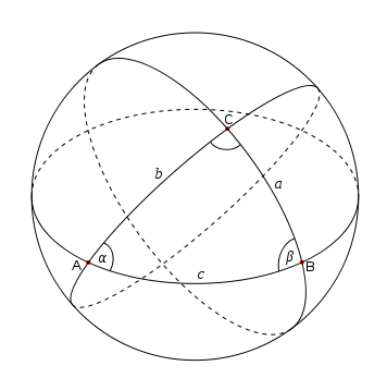
When I was in growing up, I had a copy of Handbook of Mathematical Tables and Formulas by R. S. Burington from 1940. When I first saw the book, much of it was mysterious. Now everything in the book is very familiar, and would be familiar to anyone who has gone through the typical college calculus sequence. But there is one exception: two pages on spherical trigonometry, the study of triangles drawn on a sphere.
Until recently, the only place I’d ever heard of spherical trig was Burington’s old book. I managed to find a book on spherical trig at the Rice University library, Spherical Trigonometry by J. H. D. Donnay, written in 1945. Amazon has several recent books on the spherical trig, but it appears they’re all reprints of much older books. It seems interest in teaching spherical trig died sometime after World War II.
I’m not sure why schools quit teaching spherical trig. It’s a practical subject; after all, we live on a sphere. Surveyors, navigators, and astronomers would find it useful. Somewhere along the way, solid geometry fell out of favor, and I suppose spherical trig fell out of favor with it. The standard math curriculum changed in order to make a bee line for calculus. Presumably this is to meet the needs of science and engineering students who need calculus as a prerequisite for their courses. In the process, subjects like solid geometry were squeezed out. I see the logic in the contemporary sequence, but it is interesting that the sequence was different a generation or two ago.
See Notes on Spherical Trigonometry for a list of some of the elegant identities from this now obscure area of math. For example, the interior angles of a spherical triangle must add up to more than 180°, and the area of the triangle is proportional to the amount by which the sum of these angles exceeds 180°.
The second edition of the new blog carnival Math Teachers at Play was posted this morning at Let’s Play Math.
The carnival has a wide variety of mathematical posts from elementary to advanced as well as posts on math education. Interspersed between the posts are interesting quotations such as the following from Hugo Rossi.
In the fall of 1972 President Nixon announced that the rate of increase of inflation was decreasing. This was the first time a sitting president used the third derivative to advance his case for reelection.
Two common ways to estimate the center of a set of data are the sample mean and the sample median. The sample mean is sometimes more efficient, but the sample median is always more robust. (I’m going to cut to the chase first, then go back and define basic terms like “median” and “robust” below.)
When the data come from distributions with thick tails, the sample median is more efficient. When the data come from distributions with a thin tail, like the normal, the sample mean is more efficient. The Student-t distribution illustrates both since it goes from having thick tails to having thinner tails as the degrees of freedom, denoted ν, increase.
When ν = 1, the Student-t is a Cauchy distribution and the sample mean wanders around without converging to anything, though the sample median behaves well. As ν increases, the Student-t becomes more like the normal and the relative efficiency of the sample median decreases.
Here is a plot of the asymptotic relative efficiency (ARE) of the median compared to the mean for samples from a Student-t distribution as a function of the degrees of freedom ν. The vertical axis is ARE and the horizontal axis is ν.
The curve crosses the top horizontal line at 4.67879. For values of ν less than that cutoff, the median is more efficient. For larger values of ν, the mean is more efficient. As ν gets larger, the relative efficiency of the median approaches the corresponding relative efficiency for the normal, 2/π = 0.63662, indicated by the bottom horizontal line.
The sample mean is just the average of the sample values. The median is the middle value when the data are sorted.
Since data have random noise, statistics based on the data are also random. Statistics are generally less random than the data they’re computed from, but they’re still random. If you were to compute the mean, for example, many times, you’d get a different result each time. The estimates bounce around. But there are multiple ways of estimating the same thing, and some ways give estimates bounce around less than others. These are said to be more efficient. If your data come from a normal example, the sample median bounces around about 25% more than the sample mean. (The variance of the estimates is about 57% greater, so the standard deviations are about 25% greater.)
But what if you’re wrong? What if you think the data are coming from a normal distribution but they’re not. Maybe they’re coming from another distribution, say a Student-t. Or maybe they’re coming from a mixture of normals. Say 99% of the time the samples come from a normal distribution with one mean, but 1% of the time they come from a normal distribution with another mean. Now what happens? That is the question robustness is concerned with.
Say you have 100 data points, and one of them is replaced with ∞. What happens to the average? It becomes infinite. What happens to the median? Either not much or nothing at all depending on which data point was changed. The sample median is more robust than the mean because it is more resilient to this kind of change.
Asymptotic relative efficiency (ARE) is a way of measuring how much statistics bounce around as the amount of data increases. If I take n data points and look at √n times the difference between my estimator and the thing I’m estimating, often that becomes approximately normally distributed as n increases. If I do that for two different estimators, I can take the ratio of the variances of the normal distributions that this process produces for each. That’s the asymptotic relative efficiency.
Often efficiency and robustness are in tension and you have to decide how much efficiency you’re willing to trade off for how much robustness. ARE gives you a way of measuring the loss in efficiency if you’re right about the distribution of the data but choose a more robust, more cautious estimator. Of course if you’re significantly wrong about the distribution of the data (and often you are!) then you’re better off with the more robust estimator.
In an earlier post, I quoted John Lam saying that one reason Ruby is such a good language for implementing DSLs (domain specific languages) is that function calls do not require parentheses. This allows DSL authors to create functions that look like new keywords. I believe I heard Bruce Payette say in an interview that Ruby had some influence on the design of PowerShell. Maybe Ruby influenced the PowerShell team’s decision to not use parentheses around function arguments. (A bigger factor was convenience at the command line and shell language tradition.)
In what ways has Ruby influenced PowerShell? And if Ruby is good for implementing DSLs, how good would PowerShell be?
Update: See Keith Hill’s blog post on PowerShell function names and DSLs.