Odd numbers in odd bases

My wife told me about someone on the radio yesterday discussing voluntary water rationing. People in odd-numbered houses are being asked to water their yards only on odd-numbered days. This person said “I suppose they’re talking about the last digit.”

When she told me about this, my first two thoughts were:

  1. Yes, that’s what it means to be odd.
  2. The large majority of house numbers in suburban Houston start with 1, so going by first digit would be a bad idea.

Strictly speaking, it’s a theorem that odd numbers are those that end in odd digits. The definition of an odd number is one that leaves a remainder of 1 when divided by 2. And in base 10, a number is odd if and only if it ends in an odd digit.

But what if you were using a base other than 10? If the base is even, then a number is odd if and only if the last digit is odd, just like base 10. But what if you’re using an odd base, say base 7? Then the theorem doesn’t hold. For example the number 122 in base 7 is odd, and the number 33 is even. And it’s not just the opposite of the rule for base 10 because 43 is also odd in base 7.

In an odd base, a number is odd iff it has an odd number of odd digits.

(In case you haven’t seen “iff” before, it’s an abbreviation for “if and only if.”)

So, for example, in base 7, the number 642341 is even because it contains two odd digits. And the number 744017 in base 9 is odd because it has three odd digits.

Why does this rule work? Suppose, for example, you have a 4-digit number pqrs in base b where b is odd. Then pqrs represents

p b3 + q b2 + r b + s

All the powers of b are odd, so a number like p times a power of b is odd iff p is odd. So every odd digit in the number contributes an odd number to the sum that expands what the number means. Even digits contribute even terms. A sum is odd iff it has an odd number of odd terms, so a number in an odd base is odd iff it has an odd number of odd digits.

Similar posts


A couple Python-like features in C++11

The new C++ standard includes a couple Python-like features that I ran across recently. There are other Python-like features in the new standard, but here I’ll discuss range-based for-loops and raw strings.
In Python you loop over lists rather than incrementing a loop counter variable. For example,

    for p in [2, 3, 5, 7, 11]:
        print p

Range-based for loops now let you do something similar in C++11:

    int primes[5] = {2, 3, 5, 7, 11};
    for (int &p : primes)
        cout << p << "n";

Also, Python has raw strings. If you preface a quoted string with R, the contents of the string is interpreted literally. For example,

    print "Hello\nworld"

will produce

    Hello
    world

but

    print R"Hello\nworld"

will produce

    Hello\nworld

because the \n is no longer interpreted as a newline character but instead printed literally as two characters.

Raw strings in C++11 use R as well, but they also require a delimiter inside the quotation marks. For example,

    cout << R"(Hello\nworld)";

The C++ raw string syntax is a little harder to read than the Python counterpart since it requires parentheses. The advantage, however, is that such strings can contain double quotes since a double quote alone does not terminate the string. For example,

    cout << R"(Hello "world")";

would print

    Hello "world"

In Python this is unnecessary since single and double quotes are interchangeable; if you wanted double quotes inside your string, you’d use single quotes on the outside.

Note that raw strings in C++ require a capital R unlike Python that allows r or R.

The C++ features mentioned here are supported gcc 4.6.0. The MinGW version of gcc for Windows is available here. To use C++11 features in gcc, you must add the parameter -std=c++0x to the g++ command line. For example,

    g++ -std=c++0x hello.cpp

Visual Studio 2010 supports many of the new C++ features, but not the ones discussed here.

Related links

Odd little bookshops

From Tristan Gylberd:

The smaller, the odder, the more out of the way, and the more specialized, the better. That is my philosophy on bookshops. Come to think of it, that is my philosophy on everything else too — it makes for a very interesting life unconstrained by the smothering expectations of the tyranny of fashion or popularity.

Related post: Small, local, old, and particular

Usability versus composability

Conal Elliott gave a talk at Google a while back in which he points out the tension between usability and composability, between software that is user-friendly and software that is programmer-friendly. Consumers like software that’s easy to use. But programmers like software that’s easy to compose, i.e. to combine in unanticipated ways. Users want applications; programmers want libraries. Users like GUIs; programmers like APIs.

It’s not immediately obvious that usability and composability are in tension. Why can’t you make users and programmers happy? You may be able to make some initial improvements that please both communities, but at some point their interests diverge.

Vivek Haldar picks up this theme this morning in his latest blog post. He uses “operation versus expression” to express the same idea Elliott’s idea of usability versus composability.

Combining Elliott and Haldar’s presentations, we have these contrasts.

 Usability  Composability
 Operation  Expression
 Visual / GUI  Syntactic / CLI
 Bounded  Unbounded
 Externalize knowledge  Internalize knowledge

Neither column is necessarily better. Sometimes you want to be in the left column, sometimes in the right. Sometimes you want a stereo and sometimes you want a guitar.

When I file my taxes, I want the software to be as easy to use as possible right now. There’s no long-term use to consider since I’m not going to use it again for a year, so I’ll have forgotten anything peculiar about the software by the time I open it again. But when I’m writing software, I have a different set of values. I don’t mind internalizing some knowledge of how my tools work in exchange for long-term ease of use.

Related posts

Prime telephone numbers

Michael Lugo pointed out that the telephone number 867-5309 is prime and may be the largest prime number to appear in the title of a popular song. (The song 867-5309/Jenny peaked at #4 on Billboard in 1982.)

David Radcliffe added “The phone number of Jenny’s twin sister is 8675311” because 8675309 and 8675311 are twin primes.

How likely is it for a telephone number to be prime? The Prime Number Theorem says that for large values of x, the probability that a number less than x is prime is approximately 1/log(x). Since 1/log(107) = 0.062, about 6% of phone numbers are prime.

We could try to be more accurate. We could look at the probability that a seven-digit number is prime rather than simply a number less than 107 (i.e. excluding numbers with less than seven digits). Or we could use the exact number of primes in a certain range (say using Mathematica’s PrimePi function) rather than using the Prime Number Theorem approximation. But these refinements would still give us estimates of about 6%. Note that not all seven-digit numbers have been assigned as phone numbers, so an exact calculation still gives only an approximate answer.

What about phone numbers with area codes? The Prime Number Theorem suggests about 4.3% of 10-digit numbers are prime. But the US has on the order of 300 area codes, so most 10-digit numbers are not telephone numbers. Also, area codes were not selected randomly. They were selected with a preference for smaller numbers, which means our estimate of 4.3% may be a little low. (We’d expect more prime numbers to start with small area codes.) But I imagine the area code bias has little effect.

More posts on prime numbers

System administration in remote areas

Last February I interviewed Rick Richter, CIO of Food for the Hungry, a Christian relief and development organization. This morning I spoke with Rick and was reminded of some of the challenges involved in supporting computers in poor parts of the world.

Traveling to areas most in need of relief is arduous. You may, for example, have two or three days of travel by land or water after your airplane lands. So naturally you want to do as much system administration remotely as you can.

In general you can’t expect broadband in the poorest areas, though there are some surprises. You often have to rely on satellite connections, though these are slow, unreliable, and expensive. Dial-up is preferable, if you can get it. Bandwidth may be adequate for command line access, though even then the latency is annoying. Video conferencing (e.g. for showing someone how to do something) is out of the question. So remote locations need to be mostly self-sufficient.

To read more about Food for the Hungry and their computing environment, see Why Food for the Hungry runs Ubuntu.

Designed from the inside out

The most recent episode of the Plus Maths podcast describes how the London Velodrome was designed. Being a math podcast, it focuses on the optimization problems involved in the design and the finite element modeling of the structure.

The beautiful shape of the building was not an initial goal but rather a consequence of design decisions that began with the track and worked outward.

It’s perhaps surprising, given the pragmatic design concerns of optimizing the experience of people using the velodrome, maximizing the efficiency of the building, all within the constraints of the construction methods, the design process has led to a stunningly beautiful roof that almost echos the shape of the track.

… it’s a happy by-product of the design. There was nothing intentional in the design [of the roof] that we wanted it to look like the track. … it’s the opposite if the track …

Image by Richard Davies via the Plus Math article How the velodrome found its form.

Related post: Mathematics behind the Olympic water cube

Small, local, old, and particular

Here’s an interesting thought from Rod Dreher:

Small, local, old, and particular are almost always better than big, global, new, and abstract.

Almost always better? I wouldn’t go that far. But I would say that small, local, old, and particular are often undervalued.

Since modernity is biased toward big, global, new, and abstract, giving more consideration to small, local, old, and particular can help correct our perspective.

More posts on scale

Markov chains don’t converge

I often hear people often say they’re using a burn-in period in MCMC to run a Markov chain until it converges. But Markov chains don’t converge, at least not the Markov chains that are useful in MCMC. These Markov chains wander around forever exploring the domain they’re sampling from. Any point that makes a “bad” starting point for MCMC is a point you might reach by burn-in.

Not only that, Markov chains can’t remember how they got where they are. That’s their defining property. So if your burn-in period ends at a point x, the chain will perform exactly as if you had simply started at x.

When someone says a Markov chain has converged, they may mean that the chain has entered a high-probability region. I’ll explain in a moment why that’s desirable. But the belief/hope is that a burn-in period will put a Markov chain in a high-probability region. And it probably will, but there are a couple reasons why this isn’t necessarily the best thing to do.

  1. Burn-in may be inefficient. Casting aside worries that burn-in may not do what you want, it can be an inefficient way to find a high-probability region. MCMC isn’t designed to optimize a density function but rather to sample from it.

Why use burn-in? MCMC practitioners often don’t know how to do optimization, and in any case the corresponding optimization problem may be difficult. Also, if you’ve got the MCMC code in hand, it’s convenient to use it to find a starting point as well as for sampling.

So why does it matter whether you start your Markov chain in a high-probability region? In the limit, it doesn’t matter. But since you’re averaging some function of some finite number of samples, your average will be a better approximation if you start at a typical point in the density you’re sampling. If you start at a low probability location, your average may be more biased.

Samples from Markov chains don’t converge, but averages of functions applied to these samples may converge. When someone says a Markov chain has converged, they may mean they’re at a point where the average of a finite number of function applications will be a better approximation of the thing they want to compute than if they’d started at a low probability point.

It’s not just a matter of imprecise language when people say a Markov chain has converged. It sometimes betrays a misunderstanding of how Markov chains work.

The single big jump principle

Suppose you’re playing a game where you take 10 steps of a random size. Here are two variations on the game. Which will give you a better chance of ending up far from where you started?

  1. You take your steps one at a time, starting each new step from where the last one took you.
  2. You return to the starting point after each step. After 10 turns, you go back to where your largest step took you.

Assume all steps are in the same direction. Then you’re always better off under the first rule. The sum of all your steps will be bigger than the maximum since the maximum is one of the terms in the sum.

However, depending on the probability distribution on your random steps, you may do almost as well under the second rule, taking the maximum of your steps.

If the distribution on your step size is fat-tailed (technically, subexponential) then the maximum and the sum have the same asymptotic distribution. That is, as x goes to infinity,

Pr( X1 + X2 + … + Xn > x ) ~ Pr( max(X1, X2, … , Xn) > x )

As x gets larger, the relative advantage of taking the sum rather than the maximum goes to zero. This is known as “the principle of the single big jump.” If you’re looking to make a lot of progress, adding up typical jumps isn’t likely to get you there. You need one big jump. Said another way, your total progress is about as good as the progress on your best shot.

Before you draw a life lesson from this, note that this is only true for fat-tailed distributions. It’s not true at all if your jumps have a thin-tailed distribution. But sometimes the payoffs in life’s games are fat-tailed.

What distributions are subexponential? Any fat-tailed distribution you’re likely to have heard of: Cauchy, Lévy, Weibull (with shape < 1), log-normal, etc.

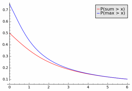
To illustrate the single jump principle, let X1 and X2 be standard Cauchy random variables. The difference between Pr( X1 + X2 > x ) and Pr( max(X1 , X2) > x ) becomes impossible to see for x much bigger than 3.

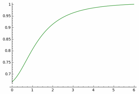
Here’s a plot of the ratio of the sum to the maximum.

The ratio tends to 1 in the limit as predicted by the single big jump principle.

I chose to use a Cauchy distribution to simplify the calculations. (The sum of two Cauchy random variables is another Cauchy. See distribution relationships.) In this case the maximum is actually larger than the sum because the Cauchy can be positive or negative. But it is still the case that the two tails converge as x increases.

More on the single big jump here.