Nonnerdy applied mathematics

From Antifragile:

There is such a thing as nonnerdy applied mathematics: find a problem first, and figure out the math that works for it (just as one acquires language), rather than study in a vacuum through theorems and artificial examples, then change reality to make it look like these examples.

This is similar to how I define very applied math in that the problem comes first, not the math.

Related posts

Visual Order and Working Order

From Two Cheers for Anarchism:

Like the city official peering down at the architect’s proposed model of a new development site, we are all prone to the error of equating visual order with working order and visual complexity with disorder. It is a natural and, I believe, grave mistake, and one strongly associated with modernism.

A few pages before the text quoted above, the author discusses planned communities that might be attractive from Superman’s perspective flying over the city but that the people on the ground find unlivable.

I thought about failed software projects with beautiful architecture diagrams and successful software projects with ugly architectural diagrams, or even no architectural diagrams. Visual order and working order may go together, but often they do not.

Personality vs experience

Be careful about saying that something isn’t a fit for your personality. Maybe it’s just outside of your experience. Several times I’ve mistaken the latter for the former.

There’s a story that when someone asked George Burns whether he could play violin, he replied “I don’t know. I haven’t tried.”

Fractal-like phase plots

Define f(z) = iz*exp(-z/sin(iz)) + 1 and g(z) = f(f(z)) + 2 for a complex argument z. Here’s what the phase plots of g look like.

The first image lets the real and imaginary parts of z range from -10 to 10.

This close-up plots real parts between -1 and 0, and imaginary part between -3 and -2.

The plots were produced with this Python code:

from mpmath import cplot, sin, exp

def f(z): return 1j*z*exp(-z/sin(1j*z)) + 1

def g(z): return f(f(z)) + 2

cplot(g, [-1,0], [-3,-2], points=100000)

The function g came from Visual Complex Functions.

Read more: Applied complex analysis

Wallpaper and phase portraits

Suppose you want to create a background image that tiles well. You’d like it to be periodic horizontally and vertically so that there are no obvious jumps when the image repeats.

Functions like sine and cosine are period along the real line. But if you want to make a two-dimensional image by extending the sine function to the complex plane, the result is not periodic along the imaginary axis but exponential.

There are functions that are periodic horizontally and vertically. If you restrict your attention to functions that are analytic except at poles, these doubly-periodic functions are elliptic functions, a class of functions with remarkable properties. See this post if you’re interested in the details. Here we’re just after pretty wallpaper. I’ll give Python code for creating the wallpaper.

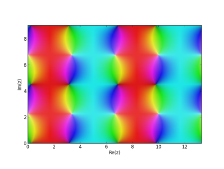
Here I’ll take a particular elliptic function sn(x). This is one of the Jacobi elliptic functions, somewhat analogous to the sine function, and use its phase portrait. Phase portraits use hue to encode the phase of a complex number, the θ value when a complex number is written in polar coordinates. The brightness of the color indicates the magnitude, the r value in polar coordinates.

Here’s the plot of sn(z, 0.2). (The sn function takes a parameter m that I arbitrarily chose as 0.2.) The plot shows two periods, horizontally and vertically. I included two periods so you could more easily see how it repeats. If you wanted to use this image as wallpaper, you could use 1/4 of the image, one period in each direction, to get by with a smaller image.

phase plot of sn(z, 0.2) - 0.2

Here’s the Python code that was used to create the image.

    from mpmath import cplot, ellipfun, ellipk
    sn = ellipfun('sn')
    m = 0.2
    x = 4*ellipk(m) # horizontal period
    y = 2*ellipk(1-m) # vertical period
    cplot(lambda z: sn(z, m) - 0.2, [0, 2*x], [0, 2*y], points = 100000)

I subtracted 0.2 from sn just to shift the color a little. Adding a positive number shifts the color toward red. Subtracting a positive number shifts the color toward blue. You could also multiply by some constant to increase or decrease the brightness.

You could also play around with other elliptic functions, described in the mpmath documentation here. And you can find more on cplot here. For example, you could supply your own function for how phase is mapped to color. The saturated colors used by default are good for mathematical visualization, but more subtle colors could be better for aesthetics.

If you make some interesting images, leave a comment with a link to your image and a description of how you made it.

Read more: Applied complex analysis

Remembering Ted Odell

I just found out this morning that Ted Odell passed away recently. He was my advisor for my undergraduate thesis and something of an informal mentor when I was in grad school. He was a kind person and a sharp mathematician.

While I was writing up my undergraduate thesis, I commented on how much help he was giving me. He quoted someone who had said that a thesis is a paper written by an advisor under the most aggravating circumstances. My intention was to study functional analysis in grad school, in part because it brought lots of areas of math together, but also in part because of the good experience I’d had working with Ted.

I remember sitting in front of the math building talking with him discussing career options. Somehow statistics came up and he said with a puzzled look on his face “Statisticians aren’t really mathematicians.” He didn’t mean that to be pejorative. He explained that statisticians have a different culture, different values, etc. Years later I would appreciate how true that is.

I also remember something he said to me about the dangers of competence. He warned me that if you’re a responsible person, willing and able to make more than a technical contribution, people will try to take advantage of you. I was flattered that he thought that could be a danger for me.

Ted and I exchanged email a while back, maybe a year ago. I was thinking about him lately and hoped to stop by his office the next time I was in Austin. I’m sorry that I won’t have that chance.

Update: Tim Gowers’ tribute to Ted Odell

Wrapping a function in a burkha

Terrific quote from Jessica Kerr via Dan North:

In an OO language you can't just pass a function around unless it's dressed in a burkha and accompanied by nouns @jessitron at #scandev

If you feel like you’re missing an inside joke, here’s an explanation.

In object oriented languages, languages that don’t simply support object oriented programming but try to enforce their vision of it, you can’t pass around a simple function. You have to pass around an object that contains the function.

Functions are analogous to verbs and objects are analogous to nouns. In contrast to spoken English where the trend is to turn nouns into verbs, OOP wraps verbs up as nouns.

“Sometimes, the elegant implementation is a function. Not a method. Not a class. Not a framework. Just a function.” — John Carmack

More posts on over-engineered software

Data calls the model’s bluff

I hear a lot of people saying that simple models work better than complex models when you have enough data. For example, here’s a tweet from Giuseppe Paleologo this morning:

Isn’t it ironic that almost all known results in asymptotic statistics don’t scale well with data?

There are several things people could mean when they say that complex models don’t scale well.

First, they may mean that the implementation of complex models doesn’t scale. The computational effort required to fit the model increases disproportionately with the amount of data.

Second, they could mean that complex models aren’t necessary. A complex model might do even better than a simple model, but simple models work well enough given lots of data.

A third possibility, less charitable than the first two, is that the complex models are a bad fit, and this becomes apparent given enough data. The data calls the model’s bluff. If a statistical model performs poorly with lots of data, it must have performed poorly with a small amount of data too, but you couldn’t tell. It’s simple over-fitting.

I believe that’s what Giuseppe had in mind in his remark above. When I replied that the problem is modeling error, he said “Yes, big time.” The results of asymptotic statistics scale beautifully when the model is correct. But giving a poorly fitting model more data isn’t going to make it perform better.

The wrong conclusion would be to say that complex models work well for small data. I think the conclusion is that you can’t tell that complex models are not working well with small data. It’s a researcher’s paradise. You can fit a sequence of ever more complex models, getting a publication out of each. Evaluate your model using simulations based on your assumptions and you can avoid the accountability of the real world.

If the robustness of simple models is important with huge data sets, it’s even more important with small data sets.

Model complexity should increase with data, not decrease. I don’t mean that it should necessarily increase, but that it could. With more data, you have the ability to test the fit of more complex models. When people say that simple models scale better, they may mean that they haven’t been able to do better, that the data has exposed the problems with other things they’ve tried.

Related posts

Robustness of equal weights

In Thinking, Fast and Slow, Daniel Kahneman comments on The robust beauty of improper linear models in decision making by Robyn Dawes. According to Dawes, or at least Kahneman’s summary of Dawes, simply averaging a few relevant predictors may work as well or better than a proper regression model.

One can do just as well by selecting a set of scores that have some validity for predicting the outcome and adjusting the values to make them comparable (by using standard scores or ranks). A formula that combines these predictors with equal weights is likely to be just as accurate in predicting new cases as the multiple-regression model that was optimal in the original sample. More recent research went further: formulas that assign equal weights to all the predictors are often superior, because they are not affected by accidents of sampling.

If the data really do come from an approximately linear system, and you’ve identified the correct variables, then linear regression is optimal in some sense. If a simple-minded approach works nearly as well, one of these assumptions is wrong.

  1. Maybe the system isn’t approximately linear. In that case it would not be surprising that the best fit of an inappropriate model doesn’t work better than a crude fit.
  2. Maybe the linear regression model is missing important predictors or has some extraneous predictors that are adding noise.
  3. Maybe the system is linear, you’ve identified the right variables, but the application of your model is robust to errors in the coefficients.

Regarding the first point, it can be hard to detect nonlinearities when you have several regression variables. It is especially hard to find nonlinearities when you assume that they must not exist.

Regarding the last point, depending on the purpose you put your model to, an accurate fit might not be that important. If the regression model is being used as a classifier, for example, maybe you could do about as good a job at classification with a crude fit.

The context of Dawes’ paper, and Kahneman’s commentary on it, is a discussion of clinical judgment versus simple formulas. Neither author is discouraging regression but rather saying that a simple formula can easily outperform clinical judgment in some circumstances.

Related posts

Negative damping

An earlier post looked at the effect of damping on free vibrations. We looked at the equation

m u'' + γ u' + k u = 0

where the coefficients m, γ, and k were all positive. But what if some of these terms are negative?

Let’s assume that m is positive. Otherwise multiply the equation above by -1. What happens if γ or k are negative?

The term γ, when positive, takes energy out of the system. A negative value of γ would be a term that adds energy, a sort of negative damping. The behavior of the solutions is determined by the eigenvalues of the system, that is the roots of the equation

m x2 + γ x + k = 0.

If γ is negative, the eigenvalues have positive real part and so the amplitude of the solutions increases exponentially. If γ2 < 4mk then the eigenvalues are complex and so the solutions have an oscillating component. If γ2 = 4mk then there is one repeated, positive eigenvalue. But if γ2 > 4mk the system has one positive and one negative eigenvalue. The solution corresponding to the negative eigenvalue decays exponentially. The other solution increases exponentially. The general solution is a linear combination of these two solutions. As time increases, only the exponentially increasing component of the solution matters because the effect of the other component goes to zero.

In theory, the solution could consist purely of the exponentially decaying component. But in practice, if there is even the tiniest component of the exponentially increasing solution, this component will eventually dominate. A numerical solution, for example, would eventually be dominated by the exponentially increasing solution.

Now what about negative springs? Instead of being a restoring force, a negative spring would be a sort of amplifier, reinforcing rather than resisting displacement. The discriminant γ2 – 4mk will be positive if k is negative. There will be no oscillation because the eigenvalues have no complex part. Also, there will be one positive and one negative eigenvalue, and so the solutions grow exponentially as described above.

Related: If you’re interested in differential equations, check out @diff_eq on Twitter.

diff_eq twitter icon