There are a couple common uses of the term distribution in math. The most familiar is probability distribution, such as a beta distribution, a Poisson distribution, etc. Less familiar but still common is distributions in the sense of generalized functions, like the Dirac delta distribution. Anybody with much exposure to math will have heard of a probability distribution. Generalized functions are common knowledge in some areas of math such as differential equations or harmonic analysis, but mathematicians in other areas, say graph theory, may not have heard of them.
This post briefly answers two questions:
- What is a distribution as in a generalized function?
- What does it have to do with a probability distribution?
Most of this post will deal with the first question, but we’ll circle back to the second question by the end.
You may have heard that a Dirac delta function δ(x) is an “infinitely concentrated” function or a point mass. Or you may have heard some of the rules for working with it, such as that it is infinite at the origin, zero everywhere else, and integrates to 1. But no function can actually do what the delta function is said to do. Measure theory will let functions take on actual infinite values, but the value of a function at a single point, even if that value is infinite, cannot matter to its integral. Even putting that aside, if you say δ(x) is infinite at 0 and integrates to 1, then how do you make sense of expressions like 2 δ? Is it twice as infinite at 0, whatever that means? Is it twice as zero everywhere else? And what on earth could it mean to take a derivative or Fourier transform of δ(x)?
Generalized functions are a way to define things like the δ distribution rigorously. They let you preserve some of the intuitive/magical properties you want while also giving rules to keep you from getting into trouble. Regarding the paragraph above, the theory will let you integrate, differentiate, and take the Fourier transform of δ(x) but it won’t let you do things like say that 2δ = δ since 2×0 = 0 and 2×∞ = ∞.
Generalized functions are just functions, but not functions of real numbers. They are linear functions that take other functions [1] and return real numbers. The functions they act on are typically called test functions. To reduce the confusion of having different kinds of functions under discussion, linear functions that act on other functions are usually called functionals. A functional is just a function, a linear function from test functions to real numbers, but it helps to give it a different name.
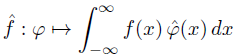
You can write the action of a distribution f on a test function φ as if it were an integral:

If f is a function, you can take the integral literally. Distributions generalize functions by associating a function with the linear operator that acts on a test function by multiplying by it and integrating.
But distributions include other kinds of linear functionals, in which case the integral expression is not literal. The δ distribution, for example, acts on a test function φ by returning φ(0). And here’s the connection to the intuitive idea of a function infinitely concentrated at 0. If a function integrates to 1, and is very concentrated near 0, then its integral when multiplied by φ is approximately φ(0). You could make this rigorous and define generalized functions as limits of functions, but that approach is something of a dead end. The theory is much simpler using the linear functional definition.
How does this let you differentiate things like the Dirac delta? In a nutshell, you take what is a theorem for ordinary functions and turn it into a definition for generalized functions. I explain this in more detail here.
So the theory of distributions lets you use your intuition regarding “infinitely concentrated” functions and such. It also lets you carry out formal calculations, such as differentiating or taking the Fourier transform of distributions. But it also keeps you out of trouble. Back to our example above, what does 2δ mean? It’s simply the linear functional that takes a test function φ and returns 2 φ(0).
Now what does all this have to do with probability distributions? You can think of a probability density function as something that exists to be integrated. You find the probability of some event (set) by integrating a probability density over it. You find the expected value of some function by multiplying that function by a probability distribution and integrating. Likewise you could think of distributions in the sense of generalized functions as things that exist to be integrated. They act on test functions by being integrated against them, or by doing things analogous to integration that are more general.
People sometimes get confused because they look at probability densities outside of integrals and try to think of them is probabilities. They’re not. They are things you integrate to get probabilities. A probability density can, for example, be larger than 1, but a probability cannot. Likewise people sometimes get confused when they think of generalized functions on their own. If you give the generalized function something to act on, you’re more likely to be guided into doing the right thing. Distributions, whether probability distributions or generalized functions, act on other things.
***
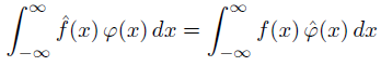
[1] The space of test functions can vary. The most common choice is infinitely differentiable functions with compact support. But for Fourier analysis, the natural space of test functions consists of infinitely differentiable functions of rapid decay, i.e. functions φ such that xn φ(x) goes to zero as x goes to ±∞ for any positive integer n.
The reason is that the Fourier transform of such a function is another function of the same kind. Test functions of compact support aren’t suited for Fourier analysis because a function with compact support cannot have a Fourier transform with compact support. It’s related to the Heisenberg uncertainty principle: the more concentrated something is in the time domain, the less concentrated it is in the frequency domain. A signal can’t be time-limited and bandlimited.
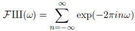
 The sha function, also known as the Dirac comb, is denoted with the Cyrillic letter sha (Ш, U+0428). This letter was chosen because it looks like how people visualize the function, a long series of vertical spikes. The function is called the Dirac comb for the same reason. This function is very important in Fourier analysis because it relates Fourier series and Fourier transforms. It relates sampling and periodization. It’s its own Fourier transform, and with a few qualifiers discussed later, the only such function.
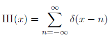


