Novel and extended floating point

My first consulting project, right after I graduated college, was developing floating point algorithms for a microprocessor. It was fun work, coming up with ways to save a clock cycle or two, save a register, get an extra bit of precision. But nobody does that kind of work anymore. Or do they?

There is still demand for novel floating point work. Or maybe I should say there is once again demand for such work.

Companies are interested in low-precision arithmetic. They may want to save memory, and are willing to trade precision for memory. With deep neural networks, for example, quantity is more important than quality. That is, there are many weights to learn but the individual weights do not need to be very precise.

And while some clients want low-precision, others want extra precision. I’m usually skeptical when someone tells me they need extended precision because typically they just need a better algorithm. And yet some clients do have a practical need for extended precision.

Some clients don’t aren’t primarily interested precision, but they’re interested in ways to reduce energy consumption. They’re more concerned with watts than clock cycles or ulps. I imagine this will become more common.

For a while it seemed that 64-bit IEEE floating point numbers had conquered the world. Now I’m seeing more interest in smaller and larger formats, and simply different formats. New formats require new math algorithms, and that’s where I’ve helped clients.

If you’d like to discuss a novel floating point project, let’s talk.

More floating point posts

Square roots of Gaussian integers

In previous post I showed how to compute the square root of a complex number. I gave as an example that computed the square root of 5 + 12i to be 3 + 2i.

(Of course complex numbers have two square roots, but for convenience I’ll speak of the output of the algorithm as the square root. The other root is just its negative.)

I chose zxiy in my example so that x² + y² would be a perfect square because this simplified the exposition.That is, I designed the example so that the first step would yield an integer. But I didn’t expect that the next two steps in the algorithm would also yield integers. Does that always happen or did I get lucky?

It does not always happen. My example was based on the Pythagorean triple (5, 12, 13). But (50, 120, 130) is also a Pythagorean triple, and the square root of z = 50 + 130i does not have integer real and imaginary parts.

At this point it will help to introduce a little terminology. A Gaussian integer is a complex number with integer real and imaginary parts. We could summarize the discussion above by saying the square root of 5 + 12i is a Gaussian integer but the square root of 50 + 120i is not.

While (5, 12, 13) and (50, 120, 130) are both are Pythagorean triples, only the first is a primitive Pythagorean triple, one in which the first two components are relatively prime. So maybe we should look at primitive Pythagorean triples.

There is a theorem going all the way back to Euclid that primitive Pythagorean triples have the form

(m² − n², 2mn, m² + n²)

where m and n are relatively prime integers and one of m and n is even.

Using the algorithm in the previous post, we can show that if x and y are the first components of a triple of the form above, then the square root of the Gaussian integer x + iy is also a Gaussian integer. Specifically we have

ℓ = m² + n²
u = √((m² + n² + m² − n²)/2) = m
v = sign(y) √((m² + n² − m² + n²)/2) = sign(y) n

This means u and v are integers and so the square root of x + iy is the Gaussian integer u + iv.

There is one wrinkle in the discussion above. Our statement of Euclid’s theorem left out the assumption that we’ve ordered the sides of our triangle so that the odd side comes first. Primitive Pythagorean triples could also have the form

(2mnm² − n², m² + n²)

and in that case our proof would break down.

Surprisingly, there’s an asymmetry between the real and imaginary parts of the number whose square root we want to compute. It matters that x is odd and y is even. For example, √(5 + 12i) is a Gaussian integer but √(12 + 5i) is not!

So a more careful statement of the theorem above is that if x and y are the first two components of a primitive Pythagorean triple, the square root of xiy is a Gaussian integer.

How to compute the square root of a complex number

Suppose you’re given a complex number

z = x + iy

and you want to find a complex number

w = u + iv

such that w² = z. If all goes well, you can compute w as follows:

ℓ = √(x² + y²)
u = √((ℓ + x)/2)
v = sign(y) √((ℓ − x)/2).

For example, if z = 5 + 12i, then ℓ = 13, u = 3, and v = 2. A quick calculation confirms

(3 + 2i)² = 5 + 12i.

(That example worked out very nicely. More on why in the next post.)

Note that ℓ ≥ |x|, and so the square roots above have non-negative arguments.

Numerical issues

I said “if all goes well” above because in floating point arithmetic, various things could go wrong. In [1], the authors point out that x² + y² could overflow. They give a more complicated algorithm that addresses the problem of overflow, and they reference a paper with an even more complicated algorithm to cover all the corner cases — NaNs, infinities, etc.

If you have access to a hypot function, it will let you compute √(x² + y²) without overflow. If you don’t have access to a hypot function, you can roll your own quickly using the algorithm here.

This may seem unnecessary. Why would you need to worry about overflow? And why would you have access to a real square root function but not a complex square root function?

If you’re using standard 64-bit floating point numbers, the hypotenuse calculation is not going to overflow as long as your arguments are less than 10154, and you can use the function csqrt from complex.h.

But if you’re using a 16-bit float or even an 8-bit float, overflow is an ever-present concern, and you might not have the math library support you’re accustomed to.

Related posts

[1] Jean-Michel Muller et al. Handbook of Floating Point Arithmetic.

Randomization audit

clipboard list of names

“How would you go about drawing a random sample?”

I thought that was kind of a silly question. I was in my first probability class in college, and the professor started the course with this. You just take a sample, right?

As with many things in life, it gets more complicated when you get down to business. Random sample of what? Sampled according to what distribution? What kind of constraints are there?

How would you select a random sample of your employees in a way that you could demonstrate was not designed to include any particular employee? How can you not only be fair, but convince people who may not understand probability that you were fair?

When there appear to be patterns in your random selections, how can you decide whether there has been an error or whether the results that you didn’t expect actually should have been expected?

How do you sample data that isn’t simply a list but instead has some sort of structure? Maybe you have data split into tables in a relational database. Maybe you have data that naturally forms a network. How can you sample from a relational database or a network in a way that respects the underlying structure?

How would you decide whether the software you’re using for randomization is adequate for your purposes? If it is adequate, are you using it the right way?

These are all questions that I’ve answered for clients. Sometimes they want me to develop randomization procedures. Sometimes they want me to audit the procedures they’re already using. They not only want good procedures, they want procedures that can stand up to critical review.

If you’d like me to design or audit randomization procedures for your company, let’s talk. You will get the assurance that you’re doing the right thing, and the ability to demonstrate that you’re doing the right thing.

Opposite of the Peter Principle

Peter Principle book cover

The Peter Principle is an idea that was developed by Lawrence Peter and expanded into a book coauthored with Raymond Hull in 1969. It says that people rise to their level of incompetence. According to the Peter Principle, competent people are repeatedly promoted until they get to a level where they’re not bad enough to fire but not good enough to promote.

I haven’t thought about the Peter Principle in a while, but I was reminded of it when I was reading One Giant Leap and was struck by this line:

He was the opposite of the Peter Principle.

What a great thing to have someone say about you. So what was the context of that line?

Jane Tindall said it about her husband Bill. The title of that chapter in One Giant Leap is “The Man Who Saved Apollo.” The author, Charles Fishman, is saying indirectly that Bill Tindall was the man who saved Apollo by getting the program’s software development effort on track. The previous chapter, “The Fourth Crew Member” explained how Apollo’s guidance computer, primitive as its hardware was by contemporary standards, was absolutely critical to the missions.

Here’s the paragraph containing the line above.

By 1966 Tindall had had years of management experience; one engineer who worked for him said that Tindall liked remaining the deputy in the divisions where he worked because it gave him more actual ability to get things done, more maneuvering room, and considerably less bureaucratic hassle. Said his wife, Jane, “He was the opposite of the Peter Principle.” [1] Tindall had the ability and experience to absorb, understand, and sort out serious technical problems, and that ability earned him the respect of his colleagues, even when they didn’t get the decision they wanted.

More Peter Principle posts

[1] No one used the term “Peter Principle” during the Apollo program because Dr. Peter had not yet coined the term yet. The quote from Jane Tindall came from Fishman interviewing her in 2016.

How probable is a probable prime?

A probable prime is a number that passes a test that all primes pass and that most composite numbers fail. Specifically, a Fermat probable prime is a number that passes Fermat’s primality test. Fermat’s test is the most commonly used, so that’s nearly always what anyone means by probable prime unless they’re more specific.

A number n is a Fermat probable prime for base b if

bn−1 = 1 (mod n).

This test isn’t conclusive, but it can be implemented efficiently and it weeds out most composite numbers. To read more on probable primes, see this post.

If a number is a probable prime, how probable is it that it really is prime? This post will briefly summarize some results from a paper [1] that makes this precise. From that paper:

… let P(x) denote the probability that an integer n is composite given that

    1. n is chosen at random with 1 < nx, n odd,
    2. b is chosen at random with 1 < b < n − 1, and
    3. n is a probable prime to the base b.

The authors give upper bounds on P(x) for x equal to various powers of 2. In particular they report

P(2250) ≤ 5.876 × 10⁻⁶

and

P(2260) ≤ 3.412 × 10⁻⁶

and so the chances that a 256-bit probable prime is composite are in the neighborhood of 4 in a million. In practice, one would test with multiple b‘s. The tests for various b‘s aren’t entirely independent, but running the tests for multiple bases does mean that fewer composite numbers slip through. There are a few pesky numbers, the Carmichael numbers, that are Fermat probable primes for nearly all bases (see footnote [2] here for more details), but these are rare.

I looked through the paper for results for larger powers of 2 to get results that would be applicable to, for example, RSA keys. The largest result explicit in the paper is

P(2330) ≤ 8.713 × 10⁻⁸

though I would like to know P(21024) and P(21536) since RSA keys are the products of (probable) primes this large. Presumably the results in [1] could be used to compute P(x) for larger values of x, but I haven’t read the paper closely enough to how much personal effort or computational effort that would require. I imagine it would be difficult or else the authors would have reported results for probable primes of the size frequently used in applications.

Related posts

[1] Jared Ducker Lichtman and Carl Pomerance. Improved error bounds for the Fermat primality test on random inputs. Mathematics of Computation. Volume 87, Number 314, November 2018, pages 2871–2890.

Negative space graph

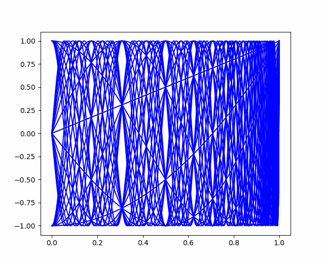
Here is a plot of the first 30 Chebyshev polynomials. Notice the interesting patterns in the white space.

Plot of first 30 Chebyshev polynomials

Forman Acton famously described Chebyshev polynomials as “cosine curves with a somewhat disturbed horizontal scale.” However, plotting  cosines with frequencies 1 to 30 gives you pretty much a solid square. Something about the way Chebyshev polynomials disturb the horizontal scale creates the interesting pattern in negative space. (The distortion is different for each polynomial; otherwise the cosine picture would be a rescaling of the Chebyshev picture.)

I found the example above in a book that referenced a book by Theodore Rivlin. There’s a new edition of Rivlin’s book coming out in August, so maybe it will say something about the gaps.

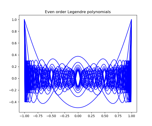
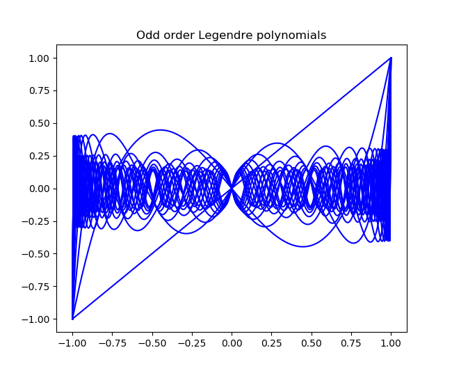
Update: Here are analogous graphs for Legendre polynomials, plotting the even and odd ordered polynomials separately. They also have conspicuous holes, but they don’t fill the unit square the way Chebyshev polynomials do.

Even order Legendre polynomials

Odd order Legendre polynomials

More on Chebyshev polynomials

Relatively prime determinants

Suppose you fill two n×n matrices with random integers. What is the probability that the determinants of the two matrices are relatively prime? By “random integers” we mean that the integers are chosen from a finite interval, and we take the limit as the size of the interval grows to encompass all integers.

Let Δ(n) be the probability that two random integer matrices of size n have relatively prime determinants. The function Δ(n) is a strictly decreasing function of n.

The value of Δ(1) is known exactly. It is the probability that two random integers are relatively prime, which is well known to be 6/π². I’ve probably blogged about this before.

The limit of Δ(n) as n goes to infinity is known as the Hafner-Sarnak-McCurley constant [1], which has been computed to be 0.3532363719…

Since Δ(n) is a decreasing function, the limit is also a lower bound for all n.

Python simulation

Here is some Python code to experiment with the math discussed above. We’ll first do a simulation to show that we get close to 6/π² for the proportion of relatively prime pairs of integers. Then we look at random 2×2 determinants.

    from sympy import gcd
    from numpy.random import randint
    from numpy import pi
    
    def coprime(a, b):
        return gcd(a, b) == 1
    
    def random_int(N):
        return randint(-N, N)
    
    def random_det(N):
        a, b, c, d = randint(-N, N, 4)
        return a*d - b*c
    
    count = 0
    N = 10000000 # draw integers from [-N, N)
    num_reps = 1000000
    
    for _ in range(num_reps):
        count += coprime(random_int(N), random_int(N))
    print("Simulation: ", count/num_reps)
    print("Theory: ", 6*pi**-2)

This code printed

    Simulation:  0.607757
    Theory:  0.6079271018540267

when I ran it, so our simulation agreed with theory to three figures, the most you could expect from 106 repetitions.

The analogous code for 2×2 matrices introduces a function random_det.

    def random_det(N):
        a, b, c, d = randint(-N, N, 4, dtype=int64)
        return a*d - b*c

I specified the dtype because the default is to use (32 bit) int as the type, which lead to Python complaining “RuntimeWarning: overflow encountered in long_scalars”.

I replaced random_int with random_det and reran the code above. This produced 0.452042. The exact value isn’t known in closed form, but we can see that it is between the bounds Δ(1) = 0.6079 and Δ(∞) = 0.3532.

Theory

In [1] the authors show that

\Delta(n) = \prod_{p \text{ prime}}\left[ 1- \left(1 - \prod_{k=1}^n (1-p^{-k})\right )^2 \right ]

This expression is only known to have a closed form when n = 1.

Related posts

[1] Hafner, J. L.; Sarnak, P. & McCurley, K. (1993), “Relatively Prime Values of Polynomials”, in Knopp, M. & Seingorn, M. (eds.), A Tribute to Emil Grosswald: Number Theory and Related Analysis, Providence, RI: Amer. Math. Soc., ISBN 0-8218-5155-1.

Sinc approximation

If a function is smooth and has thin tails, it can be well approximated by sinc functions. These approximations are frequently used in applications, such as signal processing and numerical integration. This post will illustrate sinc approximation with the function exp(−x²).

The sinc approximation for a function f(x) is given by

f(x) \approx \sum_{j=-n}^n f(jh) \, \text{sinc}\left(\frac{x - jh}{h}\right)

where sinc(x) = sin(πx)/πx.

Do you get more accuracy from sampling more densely or by sampling over a wider range? You need to do both. As the number of sample points n increases, you want h to decrease something like 1/√n and the range to increase something like √n.

According to [1], the best trade-off between smaller h and larger n depends on the norm you use to measure approximation error. If you’re measuring error with the Lebesgue p-norm [2], choose h to be

h = (\pi/2) \sqrt{q/(2n)}

where q is the conjugate exponent to p, i.e.

\frac{1}{p} + \frac{1}{q} = 1

When p = 2, q is also 2. For the sup norm, p = ∞ and q = 1.

So the range between the smallest and largest sample will be

\pi \sqrt{nq/2}

Here are a few plots to show how quickly the sinc approximations converge for exp(-x²). We’ll look at n = 1 (i.e. three sample points) , n = 2 (five sample points) and n = 4 (nine sample points). For n > 1, the sinc approximations are so good that the plots are hard to distinguish. So we’ll show the plot of exp(-x²) and its approximation for n = 1 then show the error curves.

And now the error plots.

Note that the vertical scales are different in each subplot. The error for n = 3 is two orders of magnitude smaller than the error for n = 1.

Related posts

[1] Masaaki Sugihara. Near Optimality of the Sinc Approximation. Mathematics of Computation, Vol. 72, No. 242 (Apr., 2003), pp. 767-786.

[2] The reference above doesn’t use the p-norms on the real line but on a strip in the complex plane containing the real line, and with a weight function that penalizes errors exponentially in the tails.