Accessing characters by name

snowman U+2503

You can sometimes make code more readable by using names for characters rather than the characters themselves or their code points. Python and Perl both, for example, let you refer to a character by using its standard Unicode name inside \N{}.

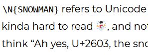
For instance, \N{SNOWMAN} refers to Unicode character U+2603, shown at the top of the post. It’s also kinda hard to read ☃, and not many people would read \u2603 and immediately think “Ah yes, U+2603, the snowman.”

A few days ago I wrote about how to get one-liners to work on Windows and Linux. Shells and programming languages have different ways to quoting and escaping special characters, and sometimes these ways interfere with each other.

I said that one way to get around problems with literal quotes inside a quoted string is to use character codes for quotes. This may be overkill, but it works. For example,

    perl -e 'print qq{\x27hello\x27\n}'

and

    python -c "print('\x27hello\x27\n')"

both print 'hello', including the single quotes.

One problem with this is that you may not remember that U+0027 is a single quote. And even if you have that code point memorized [2], someone else reading your code might not.

The official Unicode name for a single quote is APOSTROPHE. So the Python one-liner above could be written

    python -c "print('\N{APOSTROPHE}hello\N{APOSTROPHE}\n')"

This is kinda artificial in a one-liner because such tiny programs optimize for brevity rather than readability. But in an ordinary program rather than on the command line, using character names could make code easier to read.

So how do you find out the name of a Unicode character? The names are standard, independent of any programming language, so you can look them up in any Unicode reference.

A programming language that lets you use Unicode names probably also has a way to let you look up Unicode names. For example, in Python you can use unicodedata.name.

    >>> from unicodedata import name
    >>> name('π')
    'GREEK SMALL LETTER PI'
    >>> name("\u05d0") # א
    >>> 'HEBREW LETTER ALEF'

In Perl you could write

    use charnames q{ :full };
    print charnames::viacode(0x22b4); # ⊴

which prints “NORMAL SUBGROUP OF OR EQUAL TO” illustrating that Unicode names can be quite long.

Related posts

[1] How this renders varies greatly from platform to platform. Here are some examples.

Windows with Firefox:

iPad with Firefox:

iPad with Inoreader:

[2] Who memorizes Unicode code points?! Well, I’ve memorized a few landmarks. For example, I memorized where the first letters of the Latin, Greek, and Hebrew alphabets are, so in a pinch I can figure out the rest of the letters.

Pythagorean dates

The numbers that make up today’s date—12, 16, and 20—form a Pythagorean triple. That is, 12² + 16² = 20².

There won’t be any such dates next year. You could confirm this by brute force since there are only 365 days in 2021, but I hope to do something a little more interesting here.

The Mathematica function

    PowersRepresentations[n, k, p]

lists the ways to represent a number n as the sum of k pth powers. Calling PowersRepresentations[21^2, 2, 2] shows that there is no non-trivial way to write 21² as the sum of two powers; the only way is 0² + 21². You might try using the whole year rather than the last two digits, but there’s no non-trivial way to write 2021 as the sum of two powers either.

The paragraph above says that no Pythagorean triangle can have hypotenuse 21 or 2021. But could there be a Pythagorean date next year with 21 on one of the sides?

If the components of a date correspond to sides of a Pythagorean triangle, and one of the sides is 21, then the day must be on the hypotenuse because all the month numbers are less than 21, and that day must be greater than 21.

Let’s look for Pythagorean triangles with a side equal to 22, 23, …, 31 and see whether any of them have a 21 on the side.

The Mathematica command

    For[d = 22, d <= 31, d++, Print[PowersRepresentations[d*d, 2, 2]]]

returns

    {{0,22}}
    {{0,23}}
    {{0,24}}
    {{0,25},{7,24},{15,20}}
    {{0,26},{10,24}}
    {{0,27}}
    {{0,28}}
    {{0,29},{20,21}}
    {{0,30},{18,24}}
    {{0,31}}

This tells us that the only numbers from 22 to 31 that can be on the side of a Pythagorean triangle are 25, 26, 29, and 30.

The number 21 does appear in the list: (20, 21, 29) is a Pythagorean triple. But if the 29th of a month were a Pythagorean date next year, it would have to be the 20th month. Since we only have 12 months, there won’t be any Pythagorean dates next year.

The number 22, 23, and 24 can’t be written as sums of squares in a non-trivial way, so if there’s a Pythagorean date in the next few years it will have to be with the day of the month on the side. We can see from the output above that (7, 24, 25) is a Pythagorean triple, so the next Pythagorean date is 7/25/24, and the next after that is 7/24/25. And the next after that will be 10/24/26.

Incidentally, there is an algorithm for counting how many ways a number can be written as the sum of k squares, and it is implemented in Mathematica as Squares[k, n]. If you run SquaresR[2, 441] it will tell you that there are four ways to write 441 as the sum of two squares. But all four of these are trivial: (0, 21), (21, 0), (0, −21), and (−21, 0). Because every square can be written as the sum of two squares analogously, a return value of 4 means there are no non-trivial solutions.

Shells, quoting, and one-liners

The goal this post is to show how to call Perl and Python one-liners from a shell. We want to be able to use bash on Linux, and cmd or PowerShell on Windows, ideally with the same code in all three shells.

Bash

Bash interprets text inside double quotes but not in single quotes. So if you want to send a string to a program unmolested, you surround it with single quotes.

For example, suppose I want to write a Perl one-line program to print hello. This works:

    perl -e 'print "hello\n"'

The single quotes tell the shell to pass what’s inside to perl without doing anything to it.

The corresponding Python example would be

    python -c 'print("hello\n")'

and this also works.

Cmd and PowerShell

For reasons I don’t understand, the Perl example above works from cmd, but the Python example does not.

And neither example works in PowerShell. This is particularly puzzling since PowerShell follows basically the same quoting rules as bash: double quotes interpolate but single quotes do not.

Workarounds

There are ways to fix the problems with cmd and PowerShell without breaking bash.

Perl

Perl has a handy feature for avoiding confusion over quotes: you can use q{} for single quotes and qq{} for double quotes. If I write the Perl example as

    perl -e 'print qq{hello\n}'

then it works everywhere: bash, cmd, and PowerShell.

Python

Python makes no distinction between single and double quotes, so you can reverse the role of single and double quotes to avoid quoting confusion. The code

    python -c "print('hello\n')"

works everywhere.

Printing quote marks

In the previous section we said we can get around problems in Perl by using q{} and qq{}, and get around problems in Python by switching to double quotes on the outside and single quotes on the inside. But what if we wanted to print a single or double quote mark, such as printing 'hello' or "hello"?

You can escape single quotes with \' and double quotes with \", but you run into things that work on cmd but not on bash, or work on bash but not in PowerShell, etc.

One sure-fire way to make quotes work, in Perl and in Python, and on every shell we’re considering, is to denote quotes by their Unicode values, i.e. to use \x27 for single quotes and \x22 for double quotes. The one-liners

    perl -e 'print qq{\x27hello\x27\n}'

and

    python -c "print('\x27hello\x27\n')"

print 'hello' in bash, cmd, and PowerShell.

And similarly

    perl -e 'print qq{\x22hello\x22\n}'

and

    python -c "print('\x22hello\x22\n')"

print "hello" in bash, cmd, and PowerShell.

Guidelines for portable one-liners

In summary, you can avoid problems with Perl one-liners by using q{} and qq{} inside code rather than single or double quotes. For Python one-liners, you can swap single quotes and double quotes.

On Linux (bash) surround code with single quotes. On Windows (cmd and PowerShell) surround code with double quotes.

Use character codes for literal quote characters. This isn’t necessary, but if you do this you won’t have to remember how quotes and escapes work on different platforms.

Further reading

Factors of consecutive products

Pick a positive integer k and take the product of k consecutive integers greater than k. Then the result is divisible by a prime number greater than k. This theorem was first proved 128 years ago [1].

For example, suppose we pick k = 5. If we take the product

20*21*22*23*24

then it’s obviously divisible by a prime larger than 5 because 23 is one of the factors. But we could also take, for example,

32*33*34*35*36.

Although the sequence {32, 33, 34, 35, 36} doesn’t contain any primes, it contains a couple numbers with prime factors larger than 5, namely 33 = 3*11 and 34 = 2*17. Sylvester’s theorem guarantees that there will always be one number out of 5 consecutive integers that is divisible by a prime greater than 5, provided the first number is itself greater than 5.

For one more example, we can pick k = 8 and look at

140*141*142*…*147.

One of the numbers between 140 and 147 (inclusive) must be divisible by a prime greater than 8, and in fact five of them are, starting with 141 = 3*47.

In both of our examples there were multiple numbers that had a prime factor large enough to satisfy Sylvester’s theorem. Are there examples where only one number has a factor large enough? Yes, but not many.

For example, {8, 9} is a pair of consecutive integers, only one of which has a prime factor bigger than 2. And {8, 9, 10} is an example of 3 consecutive integers, only one of which has a prime factor larger than 3. I wrote a program to search for examples with k = 4 and didn’t find any.

In any case, a theorem dating back to 1897 [2] proves that there could only be finitely many examples for k > 2. Lehmer extends the results [2] in his paper [3].

***

[1] J. J. Sylvester, On arithmetical series, Messenger Math., 21 (1892) 1-19, and 87-120; Collected Mathematical Papers, 4 (1912) 687-731.

[2] G. St0rmer, Quelques theoremes sur l’equation de Pell x² − Dy² = ± 1 et leurs applications,
Skr. Norske Vid. Akad. Oslo, I no. 2 (1897).

[3] D. H. Lehmer, The Prime Factors of Consecutive Integers, The American Mathematical Monthly , Feb., 1965, Vol. 72, No. 2, Part 2, pp. 19-20.

Four meanings of ^

Logic vs C

I recently made a mistake because I interpreted the symbol ^ in the wrong context. I saw an expression of the form a ^ b and thought of the ^ as AND, as in logic, but the author’s intent was XOR, as in C.

How else might someone misinterpret the ^ operator? Here are a couple more possibilities. They’re sufficiently different contexts that they’re more like puns than likely mistakes.

Wedge products

The ^ symbol is also used in mathematics for wedge products of differential forms. Surely that’s completely different from bit twiddling, right? Actually it’s similar.

The wedge product of a differential form with itself is 0, i.e.

x ^ x = 0

for any differential form x. But that’s also true if you interpret x as a Boolean variable and ^ as XOR.

Another property of wedge products is that products are alternating:

x ^ y = − (y ^ x).

That doesn’t look right for bits, but it is. If you think of 0 and 1 as elements of a binary field, i.e. GF(2), then – means additive inverse. But everything is its own additive inverse in this context, so

x ^ y = y ^ x = − (y ^ x)

for bits with XOR just as for differential forms with exterior product.

Not everything from wedge products works for bits, however. For wedge products, any repetition in terms makes the product zero, whereas for XOR it’s only even numbers of replication that always equal zero. For example,

x ^ x ^ x = 0

is always true for differential forms, but is not true for bits if x = 1.

Exponents

The ^ symbol is also used for exponents, such as x ^ y in LaTeX for xy.

In the context of bits, ^ is the same as ≥. That is, for binary variables x and y, xy is 1 if and only if x ≥ y.

You might object that I’m moving back and forth freely between thinking of 0 and 1 as elements of a field and as truth values, but this post is all about being a little sloppy with context.

The Crown and The Planets

I first heard the hymn “I Vow to Thee, My Country” while watching the first season of The Crown [1]. I assume the hymn is familiar in the UK, but it is not in America as far as I know.

When I say I first heard the hymn, I mean that I first heard it as a hymn with words. I thought the tune sounded familiar, and that it reminded me of The Planets by Holst.

I’ve started watching the latest season of The Crown and once again I heard the hymn [2], so this time I looked into it more. The tune does indeed come from The Planets, specifically from the middle of the Jupiter movement.

With a little searching I found the sheet music to the hymn.

Sheet music for the tune Thaxted

This brought up more things I’ve long meant to look into. As a child I remember cryptic notations around hymns, such as “Thaxted 13.13.13 D” above, and never knew what they meant.

Tunes have names independent of the hymns they appear in, but these tune names were, and still are, completely unfamiliar to me. For example, the hymn “Amazing Grace” has the tune “McIntosh,” though I don’t imagine many people know that.

In the example here, “Thaxted” is the name of the melody from Jupiter when it is used as a hymn. The name comes from the English town of Thaxted where Holst lived. Perhaps there are other hymns that use the same tune.

Now what about the mysterious numbers 13.13.13? They mean that the hymn is built out of groups of three lines, each with 13 syllables. The hymn Once in Royal David’s City is marked 87 87 77, meaning the hymn has three phrases, the first two alternating lines of 8 and 7 syllables, and the last having two lines of 7 syllables each.

From what I’ve read, the “D” in “13.13.13 D” stands for double meter, which I would take to mean 2/4, but the tune is clearly in 3/4, so I’m not sure what the D means.

Update: The D means the entire pattern is doubled, not that the meter is double time. Thaxted has six lines, in two groups of three. Thanks to Michael Lugo for letting me know via Twitter.

***

[1] S1E1 10:00

[2] S4E3 40:30


Predictive probability for large populations

Suppose you want to estimate the number of patients who respond to some treatment in a large population of size N and what you have is data on a small sample of size n.

The usual way of going about this calculates the proportion of responses in the small sample, then pretends that this is the precisely known proportion, and applies it to the population as a whole. This approach underestimates the uncertainty in the final estimate because it ignores the uncertainty in the initial estimate.

A more sophisticated approach creates a distribution representing what is known about the proportion of successes based on the small sample and any prior information. Then it estimates the posterior predictive probability of outcomes in the larger population based on this distribution. For more background on predictive probability, see my post on uncertainty in a probability.

This post will look at ways to compute predictive probabilities using the asymptotic approximation presented in the previous post.

Suppose your estimate on the probability of success, based on your small sample and prior information, has a Beta(α, β) distribution. Then the predictive probability of s successes and f failures is

 {s + f \choose s} \frac{B(s + \alpha, f + \beta)}{B(\alpha, \beta)}

The beta functions in the numerator and denominator are hard to understand and hard to compute, so we would like to replace them with something easier to understand and easier to compute.

We begin by expanding all the terms involving s and f in terms of gamma functions.

\frac{1}{B(\alpha,\beta)} \frac{\Gamma(s+f+1)}{\Gamma(s+1)\, \Gamma(f+1)} \frac{\Gamma(s+\alpha)\, \Gamma(f+\beta)}{\Gamma(s+f+\alpha+\beta)}

By rearranging the terms we can see three examples of the kind of gamma function ratios estimated in the previous post.

\frac{1}{B(\alpha,\beta)} \frac{\Gamma(s+\alpha)}{\Gamma(s+1)} \frac{\Gamma(f+\beta)}{\Gamma(f+1)} \frac{\Gamma(s+f+1)}{\Gamma(s+f+\alpha+\beta)}

Now we can apply the simplest approximation from the previous post to get the following.

\frac{s^{\alpha-1} f^{\beta-1} (s +f)^{1 - \alpha-\beta-1}}{B(\alpha, \beta)}

We can make this approximation more symmetric by expanding Beta(α, β) in terms of factorials:

 \frac{(\alpha + \beta-1)!}{(\alpha-1)!\, (\beta-1)!} \,\,\frac{s^{\alpha-1} f^{\beta-1}}{(s+f)^{\alpha+\beta-1}}

We saw in the previous post that we can make our asymptotic approximation much more accurate by shifting the arguments a bit, and the following expression, while a little more complicated, should be more accurate.

\frac{(\alpha + \beta-1)!}{(\alpha-1)!\, (\beta-1)!} \,\, \frac{ \left(s + \tfrac{\alpha}{2}\right)^{\alpha-1} \left(f + \tfrac{\beta}{2}\right)^{\beta-1} }{ \left(s +f + \tfrac{\alpha+\beta}{2}\right)^{\alpha+\beta-1} }

This should be accurate for sufficiently large s and f, but I haven’t tested it numerically and wouldn’t recommend using it without doing some testing first.

Asymptotic series for gamma function ratios

Applications of statistics often require working with

for large x and fixed α and β.

The simplest approximation to this ratio of gamma functions is

You can do a little better [1] with

(x + c)^{\alpha - \beta}

where c = (α + β − 1)/2.

To get more accuracy we’ll need more terms. Tricomi and Erdélyi worked out the full asymptotic series 70 years ago:

\frac{\Gamma(x+\alpha)}{\Gamma(x+\beta)} \sim \sum_{n=0}^\infty {\alpha-\beta\choose n}B_n^{\alpha-\beta+1}(\alpha) x^{\alpha - \beta - n}

Here Bnλ is the “generalized Bernoulli polynomial,” a.k.a. the Nørlund polynomial [3].

There’s no simple way to state the coefficients in the series above. The expression in terms of Nørlund polynomials is compact, but then the Nørlund polynomials are a bit complicated to define. The can be calculated in Mathematica with NorlundB, and so the coefficients would be

     Binomial[α-β, n] NorlundB[n, α-β+1, α]

in Mathematica.

Let’s see how the various approximations compare in an example.

    {α, β} = {3.4, 5.6}
    f[x_] := Gamma[x+α]/Gamma[x+β]
    f1[x_] = x^(α-β)
    f2[x_] = (x + (α+β-1)/2)^(α-β)
    f3[x_] = Sum[Binomial[α-β, n]
                 NorlundB[n, α-β+1, α]
                 x^{α-β-n}, {n, 0, 2}]

We can plot the exact function f and its approximations with

    LogPlot[{f[x], f1[x], f2[x], f3[x]}, {x, 10, 15}, 
          PlotLabels -> Automatic]

This gives the following.

It’s interesting that the approximation f2 works really well and is the most accurate approximation over the range shown. For large enough x, say x = 1000, the series approximation f3 will be more accurate.

***

[1] A. Laforgia, P. Natalini. On the asymptotic expansion of a ratio of gamma functions. Journal of Mathematical Analysis and Applications. Volume 389, Issue 2, 15 May 2012, pp. 833-837.

[2] F. G. Tricomi, A. Erdélyi. The asymptotic expansion of a ratio of gamma functions. Pacific J. Math. 1 (1951), pp. 133-142.

[3] The authors in [1] quote this formula from [2] but leave out the binomial coefficient. Note that the binomial coefficient parameters are not necessarily positive integers and so the binomial coefficients should be interpreted in the sense of the most general definition.

Redundant Residue Number Systems

You can uniquely represent a large number by its remainders when divided by smaller numbers, provided the smaller numbers have no factors in common, and carry out arithmetic in this representation. Such a representation is called a Residue Number System (RNS).

In the 1960s people realized RNSs could be useful in computer arithmetic. The original papers are now hard to find, but you can find a summary of some of their ideas here. We will give examples working in a particular RNS below.

When you work with remainders by more numbers than necessary, you have a Redundant Residue Number System (RRNS) that provides error detection and correction. We will also demonstrate this with an example.

RNS example

To be concrete, we’ll use the remainders by 199, 233, 194, and 239 to represent numbers, following the work of C. W. Hastings and R. W. Watson referenced in the link cited above.

Let M = 199*233*194*239. Any non-negative integer less than M can be specified by its remainders mod 199, 233, 194, and 239.

The following Python code generates a random number less than M, represents it by its remainders, and then recovers the original number from the remainders using the Chinese Remainder Theorem.

    from random import randrange
    from sympy import prod
    from sympy.ntheory.modular import crt

    moduli = [199, 233, 194, 239]
    M = prod(moduli)

    x = randrange(M)
    remainders = [x % m for m in moduli]
    # See footnote [1]
    y = crt(moduli, remainders, symmetric=False)[0]

    print(x)
    print(remainders)
    print(y)

This printed

    1119075671
    [166, 204, 57, 235]
    1119075671

You can add, subtract, and multiply numbers by carrying out the corresponding operations on their remainders. There are three advantages to this.

First, you can work with smaller numbers. In our example, all the moduli are 8-bit numbers; we can carry out arithmetic on 32-bit numbers [2] by only working directly with 8-bit numbers. We could use the same idea to represent extremely large numbers by their remainders via 64-bit integers.

Second, we can do our calculations in parallel, working with each of our remainders at the same time.

Third, there are no carries. There’s no need to keep track of whether component calculations overflow.

The following code shows how we can add two numbers via their remainders.

    a = randrange(M//2)
    b = randrange(M//2)

    arem = [a % m for m in moduli]
    brem = [b % m for m in moduli]
    crem = [z[0] + z[1] for z in zip(arem, brem)]
    c = crt(moduli, crem, symmetric=False)[0]

    print(a + b)
    print(c)

When I ran this code, it printed 832537447 twice.

RRNS

Now we get to the redundant part. Suppose we add more numbers to our list of moduli, larger than the previous numbers and relatively prime to all of them and to each other. Now working modulo this larger list of numbers, we have more information than we need. If the results we get from using various subsets of the list of moduli are inconsistent, we’ve detected an error. And with enough extra information, we can correct the error.

Watson and Hastings added 251 and 509 in their example, and so we’ll do the same.

As before, we will generate a couple random numbers and represent them via their remainders, though now by a longer list of remainders. We will deliberately corrupt one of the component sums and then compute their sum using different choices of four moduli from the set of six.

    xmoduli = [199, 233, 194, 239, 251, 509]
    a = randrange(M//2)
    b = randrange(M//2)
    aremx = [a % m for m in xmoduli]
    bremx = [b % m for m in xmoduli]
    cremx = [z[0] + z[1] for z in zip(aremx, bremx)]
    cremx[1] += 13

    c0 = crt(xmoduli[:4], cremx[:4], symmetric=False)[0]
    c1 = crt(xmoduli[2:], cremx[2:], symmetric=False)[0]
    c2 = crt(xmoduli[:2] + xmoduli[4:], cremx[:2] + cremx[4:], symmetric=False)[0]
    print(c0, c1, c2)

This will return three different answers, so we know that there has been an error. When I ran it I got 70315884, 819846513, and 890162397. If you run the code yourself you’ll get different answers since you’ll generate different random numbers.

Now how do we correct the error? Suppose we know there has only been one error (or more realistically, we are willing to assume that the probability of two errors is tolerably small). Then one of the results above must be correct: the first sum excludes the last two moduli, the second excludes the first two, and the last excludes the middle two. One of them must exclude the error.

The first calculation based on a different subset of moduli that gives one of the results above is correct. The code

    c3 = crt(xmoduli[:1]+xmoduli[2:5], cremx[:1] + cremx[2:5], symmetric=False)[0]
    print(c3)

produced 890162397, matching the third sum above, so we know that eliminating the second modulus gives the correct answer. We’ve found the correct answer, and we’ve discovered which component was corrupted.

***

[1] A couple things about the call to crt require explanation. We set symmetric to False in order to get a positive return value. Otherwise we might get a value that is correct mod M but negative. Also, crt returns not just the solution we’re after but a pair consisting of the solution and the product of the moduli. We take the first element of the pair with [0] to get the part we’re interested in.

[2] Not all 32-bit numbers. with any numbers less than M, and M is between 231 and 232.

Ruling out gaps in the list of Mersenne primes

The largest known primes are Mersenne primes, in part because the Lucas-Lehmer algorithm makes it more efficient to test Mersenne numbers for primality than to test arbitrary numbers. These numbers have the form 2n − 1.

Trend in Mersenne primes

The Great Internet Mersenne Prime Search (GIMPS) announced today that they have tested whether 2n – 1 is prime for all values of n less than 100,000,000 [1]. More specifically, they’ve tested each exponent at least once, though they’d like to test each exponent twice before giving up on it.

If we assume all of their initial calculations are correct, we can say, for example, that 282,589,933 − 1 is the 51st Mersenne prime. Before we had to say that it was the 51st known Mersenne prime because there could be a smaller, undiscovered Mersenne prime, in which case 282,589,933 − 1 might be the 52nd Mersenne prime. Mersenne primes have not always been discovered in order. For example, the 29th Mersenne prime was discovered after the 30th and 31st such numbers.

So for now, again assuming all the GIMPS calculations have been correct, we know all Mersenne primes less than 2100,000,000, and there are 51 of them.

Related posts

[1] There’s no need to test every value of n. We know that if 2n − 1 is prime, then n is prime. So we only need to check prime values of n.