The Latin of Linux

One reason people study Latin is that it is the ancestor of many modern languages. English derives from West Germanic languages, not from Latin, but much of English vocabulary, perhaps as much as 60%, derives from Latin, either directly or indirectly through French.

Knowing a bit of Latin makes sense of many things that would otherwise seem completely arbitrary, such as why the symbols for gold, silver, and lead are Au, Ag, and Pb respectively.

Similarly, ed(1) is the Latin of Linux [1]. Many conventions in command line utilities follow conventions that go back to the ed(1) line editor. They may go back even further. Just as Latin didn’t come out of nowhere, neither did ed(1), but you can’t go back indefinitely. It’s convenient to start history somewhere, and this post will start with ed(1) just as much discussion of Western linguistics starts with Latin.

The following are features of ed(1) that live on in sed, awk, grep, vi, perl, bash, etc.

  1. Using slashes to delimit regular expressions
  2. Using $ to indicate the end of a line or the end of a file
  3. The pattern of specifying address + action or address range + action
  4. Using regular expressions as address ranges
  5. Using \1, \2, etc to refer to regex captures
  6. Using & to refer to the entire matched text
  7. The g/regexp/command pattern
  8. Using p for printing lines, as in g/re/p
  9. The commands a, c, d, i, j, l, p, q, r, and w in vi
  10. ! for shell escape


[1] Because the name “ed” is so short, and looks so much like the name Ed, it’s convenient to use its full Unix name ed(1). The parenthesized number is used to disambiguate different things that have the same name, such as the user command kill(1) and the system call kill(2). There is no ed(2) or any other higher-numbered ed. The number is there to make the name stand out, not to disambiguate anything.
Naively summing an alternating series

Suppose you run across the power series for the exponential function and decide to code it up. Good idea: you’ll probably learn something, though maybe not what you expect.

Maybe you decide a tolerance of 10−12 is good enough, and so you sum the terms until the next term to add is below the tolerance.

from math import factorial, exp

def naive_exp(x):
    tolerance = 1e-12
    s = 0
    n = 0
    while True:
        delta = x**n / factorial(n)
        s += delta
        if abs(delta) < tolerance:
            return s
        n += 1

You want to try your program out, so you compute e by calling the function at 1. If you compare this to calling exp(1) you find that you got all the digits correct.

Now you try computing exp(-20). Calling naive_exp(-20) gives

    5.47893091802112e-10

but calling exp(-20) gives

    2.061153622438558e-09

Don’t brush things like this as flukes or compiler bugs [1]. This is your golden opportunity to learn something.

Maybe you add a print statement to see the intermediate values of the sum stored in the variable s. If you do, you’ll see that the partial sums oscillate wildly before settling down.

Maybe that seems wrong, but then you look more carefully at the series. The nth term is xn/n!. Since x is negative, the terms alternate in sign. And the absolute values of the term get bigger before they get smaller. When x = −20, each numerator is 20 times larger than the previous, and each denominator is n times larger than the previous. So the terms will get bigger until n > 20. So the wild oscillations are real, not a bug.

The largest partial sum is 21822593.77927747 in absolute value. You know that exp(−20) is a very small number, so there’s going to have to be a lot of cancellation before the partial sums settle down to a small number. Maybe you’ve heard that cancellation is where numerical calculations lose precision. If not, now you know!

Look again at the largest partial sum. There are eight figures to the right of the decimal point. The code is printing out results to as much precision as it has, so the error at this point is on the order of 10−8. We’re trying to compute a number on the order of 10−9, and if any digits in our result are correct, it would be a coincidence.

If you go back and try your code on x = −22, the result is even worse, giving a negative result for a quantity that for theoretical reasons cannot be negative. But you can see why: you’re asking the code to compute a number that is closer to zero than the accuracy of the code.

Computers don’t represent numbers in base 10 internally, but the argument above is sufficient in this case. If you want to dig deeper, look into the anatomy of a floating point number.

There is a simple way around the problem above, but discovering it sooner would short-circuit the learning process. You could calculate exp(−20) as 1/exp(20) and avoid all the cancellation because the series for exp(20) does not alternate.


[1] Compilers do have bugs occasionally, but it’s orders of magnitude more likely that something is wrong with your code.

Online (one-pass) algorithms

Canonical example

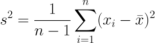
The sample variance of a set of numbers is defined in terms of the sum of the squared distances from each point to the mean.

s^2 = \frac{1}{n-1}\sum_{i=1}^n (x_i -\bar{x})^2

So it would seem that you first need to calculate the mean, then go back and compute the squared differences from the mean. And yet sample variance can be computed in one pass through the data.

You’ll find two equivalent equations in statistics books: the one described above and another based on the sum of the data points and the sum of the data points squared.

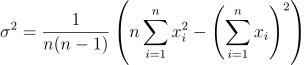
s^2 = \frac{1}{n(n-1)}\left(n\sum_{i=1}^n x_i^2 -\left(\sum_{i=1}^n x_i\right)^2\right)

While this equation is theoretically correct, it is numerically unstable. Code that directly implements this equation can return a negative value for a quantity that is theoretically positive. I’ve seen this happen with real data, causing a program to crash when taking the square root of the variance to get the standard deviation.

However, there is an algorithm that computes mean and variance in one pass that is accurate and numerically stable. This algorithm was developed by B. P. Welford in 1962. I discuss Welford’s algorithm and give code for implementing it here.

Online algorithms

Welford’s algorithm is known in computer science as an “online” algorithm. This term was coined well before the Internet. For example, see the paper [1] from 1965.

But of course now “online” means something else, and so the technical and colloquial uses of “online algorithm” have split. Technical literature uses the phrase to describe the kinds of algorithms in this post. Most people would take “online algorithm” to mean code that runs on a remote server. You may see “streaming algorithm” as a contemporary technical term, but I’d still search on “online algorithm” to find papers.

Computing higher moments online

Welford’s algorithm computes the first two moments, mean and variance, of a data set online. It is also possible to compute skewness and kurtosis online, as well as higher moments.

Online regression

Simple linear regression is closely related to calculating mean and variance, and it is possible to compute simple regression coefficients online. I have some old notes on this here.

This post was motivated by an email asking me about multiple regression. It is also possible to compute multiple regression coefficients online, but I haven’t done this. I found a couple references, [2] and [3], but I have not read them. There is a simple procedure for two predictor variables but I believe things get a little more complicated with three or more predictors, requiring a recursive least squares algorithm.

Related posts

The notion of online algorithms is closely related to the notion of a fold in functional programming. Here are several posts on computing things with folds.

[1] One-Tape, Off-Line Turing Machine Computations by F. C. Hennie. Information and Control. 8, 553-578 (1965). Available here. In this paper Hennie writes “In an on-line computation the input data are supplied to the machine, one symbol at a time, at a special input terminal. … In an off-line computation all of the input symbols are written on one of the machine’s tapes prior to the start of the computation.

[2] Arthur Albert and Robert W. Sittler, “A Method for Computing Least Squares Estimators that Keep Up with the Data,” Journal of the Society for Industrial and Applied Mathematics, Series A: Control, 3(3), 384–417, 1965. DOI: 10.1137/0303026.

[3] Petre Stoica and Per Ashgren. Exact initialization of the recursive least-squares algorithm. Int. J. Adapt. Control Signal Process. 2002; 16:219&ndashh;230.

Calculating the expected range of normal samples

The previous post looked at the expected IQ range in a jury of 12. This post will look more generally at computing the expected range of n samples from a N(0, 1) random variable. This will give the expected range in units of σ, i.e. multiply the results by σ if your σ isn’t 1.

As mentioned in the previous post, the expected range is given by

d_n = 2n \int_{-\infty}^\infty \Phi(x)^{n-1} \, x\,\phi(x) \, dx

where φ and Φ are the PDF and CDF of a standard normal. The integral can be calculated in closed form for n ≤ 5, but in general it requires numerical integration [1].

The following Python code can compute dn.

from scipy.stats import norm
from scipy.integrate import quad
import numpy as np

def d(n):
    integrand = lambda x: x*norm.pdf(x)*norm.cdf(x)**(n-1)
    res, info = quad(integrand, -np.inf, np.inf)
    return 2*n*res

For large n we have the asymptotic approximation

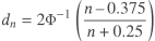
d_n = 2 \Phi^{-1}\left( \frac{n \,–\, 0.375}{ n + 0.25} \right)

which we could implement in Python by

def approx(n):
    return 2*norm.ppf((n - 0.375)/(n + 0.25))

For very large n the asymptotic expression may be more accurate than the integral due to numerical integration error.

Here are a few example values.

|-----+-------|
|   n |   d_n |
|-----+-------|
|   2 | 1.128 |
|   3 | 1.693 |
|   5 | 2.326 |
|  10 | 3.078 |
|  12 | 3.258 |
|  23 | 3.858 |
|  50 | 4.498 |
| 100 | 5.015 |
|-----+-------|

[1] Order Statistics by H. A. David. John Wiley & Sons. 1970.

Recovering the state of xorshift128

I’ve written a couple posts lately about reverse engineering the internal state of a random number generator, first Mersenne Twister then lehmer64. This post will look at xorshift128, implemented below.

import random

# Seed the generator state
a: int = random.getrandbits(32)
b: int = random.getrandbits(32)
c: int = random.getrandbits(32)
d: int = random.getrandbits(32)

MASK = 0xFFFFFFFF

def xorshift128() -> int:
    global a, b, c, d

    t = d
    s = a

    t ^= (t << 11) & MASK t ^= (t >>  8) & MASK
    s ^= (s >> 19) & MASK

    a, b, c, d = (t ^ s) & MASK, a, b, c

    return a

Recovering state

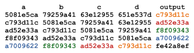
Recovering the internal state of the generator is simple: it’s the four latest outputs in reverse order. This is illustrated by the following chart.

 a b c d output 5081e5ca 79259a41 63e12955 651e537d c793d11c c793d11c 5081e5ca 79259a41 63e12955 ad52e33a ad52e33a c793d11c 5081e5ca 79259a41 f8f09343 f8f09343 ad52e33a c793d11c 5081e5ca a7009622 a7009622 f8f09343 ad52e33a c793d11c fe42a8ef

This means that once we’ve seen four outputs, we can predict the rest of the outputs. The following code demonstrates this.

Let’s generate five random values.

out = [xorshift128() for _ in range(5)]

Running

print(hex(out[4]))

shows the output 0xc3f4795d.

If we reset the state of the generator using the first four outputs

d, c, b, a, _ = out
print(hex(xorshift128()))

we get the same result.

Good stats, bad security

Mersenne Twister and lehmer64 have good statistical properties, despite being predictable. The xorshift128 generator is even easier to predict, but it also has good statistical properties. These generators would be fine for many applications, such as Monte Carlo simulation, but disastrous for use in cryptography.

The post on lehmer64 mentioned at the end that the internal state of PCG64 can also be recovered from its output. However, doing so requires far more sophisticated math and thousands of hours of compute time. Still, it’s not adequate for cryptography. For that you’d need a random number generator designed to be secure, such as ChaCha.

So why not just use a cryptographically secure random number generator (CSPRNG) for everything? You could, but the other generators mentioned in this post use less memory and are much faster. PCG64 occupies an interesting middle ground: simple and fast, but not easily reversible.

Initialize and print 128-bit integers in C

If you look very closely at my previous post, you’ll notice that I initialize a 128-bit integer with a 64-bit value. The 128-bit unsigned integer represents the internal state of a random number generator. Why not initialize it to a 128-bit value? I was trying to keep the code simple.

A surprising feature of C compilers, at least of GCC and Clang, is that you cannot initialize a 128-bit integer to a 128-bit integer literal. You can’t directly print a 128-bit integer either, which is why the previous post introduces a function print_u128.

The code

__uint128_t x = 0x00112233445566778899aabbccddeeff;

Produces the following error message.

error: integer literal is too large to be represented in any integer type

The problem isn’t initializing a 128-bit number to a 128-bit value; the problem is that the compiler cannot parse the literal expression

0x00112233445566778899aabbccddeeff

One solution to the problem is to introduce the macro

#define U128(hi, lo) (((__uint128_t)(hi) << 64) | (lo))

and use it to initialize the variable.

__uint128_t x = U128(0x0011223344556677, 0x8899aabbccddeeff);

You can verify that x has the intended state by calling print_u128 from the previous post.

void print_u128(__uint128_t n)
{
    printf("0x%016lx%016lx\n",
           (uint64_t)(n >> 64),      // upper 64 bits
           (uint64_t)n);             // lower 64 bits
}

Then

print_u128(x);

prints

0x00112233445566778899aabbccddeeff

Update. The code for print_u128 above compiles cleanly with gcc but clang gives the following warning.

warning: format specifies type 'unsigned long' but the argument has type 'uint64_t' (aka 'unsigned long long') [-Wformat]

You can suppress the warning by including the inttypes header and modifying the print_u128 function.

Here’s the final code. It compiles cleanly under gcc and clang.

#include <stdio.h>
#include <stdint.h>
#include <inttypes.h>
#define U128(hi, lo) (((__uint128_t)(hi) << 64) | (lo))

void print_u128(__uint128_t n)
{
    printf("0x%016" PRIx64 "%016" PRIx64 "\n",
           (uint64_t)(n >> 64),
           (uint64_t)n);
}

int main(void)
{
    __uint128_t x = U128(0x0011223344556677, 0x8899aabbccddeeff);
    print_u128(x);
    return 0;
}

Hacking the lehmer64 RNG

A couple days ago I wrote about hacking the Mersenne Twister. I explained how to recover the random number generator’s internal state from a stream of 640 outputs.

This post will do something similar with the lehmer64 random number generator. This generator is very simple to implement. Daniel Lemire found it to be “the fastest conventional random number generator that can pass Big Crush,” a well-respected test for pseudorandom number generators.

Implementing lehmer64

The lehmer64 generator can be implemented in C by

__uint128_t g_lehmer64_state;

uint64_t lehmer64() {
    g_lehmer64_state *= 0xda942042e4dd58b5ULL;  
  return g_lehmer64_state >> 64;
}

The analogous code in Python would have to simulate the overflow behavior of a 128-bit integer by reducing the state mod 2128 after the multiplication.

Reverse engineering lehmer64 is easier than reverse engineering the Mersenne Twister because only three outputs are needed. However, the theory behind the exploit is more sophisticated. See [1].

The following code sets the state to an arbitrary initial seed value and generates three values.

#include <stdio.h>
#include <stdint.h>

int main(void)
{
    g_lehmer64_state = 0x4789499d78770934; // seed
    for (int i = 0; i < 3; i++) {
        printf("0x%016lx\n", lehmer64());
    }

    return 0;
}

The code prints the following.

0x3d144d12822bcc2e
0x85a67226191a568d
0x53e803dffc88e8f8

Exploiting lehmer64

Here is Python code for recovering the state of the lehmer64 generator given in [1].

def reconstruct(X):
    a = 0xda942042e4dd58b5
    r = round(2.64929081169728e-7 * X[0] + 3.51729342107376e-7 * X[1] + 3.89110109147656e-8 * X[2])
    s = round(3.12752538137199e-7 * X[0] - 1.00664345453760e-7 * X[1] - 2.16685184476959e-7 * X[2])
    t = round(3.54263598631140e-8 * X[0] - 2.05535734808162e-7 * X[1] + 2.73269247090513e-7 * X[2])
    u = r * 1556524 + s * 2249380 + t * 1561981
    v = r * 8429177212358078682 + s * 4111469003616164778 + t * 3562247178301810180
    state = (a*u + v) % (2**128)
    return state

Let’s call reconstruct with the output of our C code.

X = [0x3d144d12822bcc2e, 0x85a67226191a568d, 0x53e803dffc88e8f8]
print( hex( reconstruct(X) ) )

This prints

0x3d144d12822bcc2e1b81101c593761c4

Now for the confusing part: at what point is the number above the state of the generator? Is it the state before or after generating the three values? Neither! It is the state after generating the first value.

We can verify this by modifying the C code as follows and rerunning it.

void print_u128(__uint128_t n)
{
    printf("0x%016lx%016lx\n",
           (uint64_t)(n >> 64),      // upper 64 bits
           (uint64_t)n);             // lower 64 bits
}

int main(void)
{
    g_lehmer64_state = 0x4789499d78770934; // seed
    for (int i = 0; i < 3; i++) {
        printf("0x%016lx\n", lehmer64());
        printf("state: ");
        print_u128(g_lehmer64_state);
    }
 
    return 0;
}

The main goal of [1] is to recover the state of the PCG generator, not the lehmer64 generator. The latter was a side quest. Recovering the state of PCG64 is much harder; the authors estimate it takes about 20,000 CPU-hours. The paper shows that a technique used as part of pursuing their main goal can quickly recover the lehmer64 state.

Related posts

[1] Charles Bouillaguet, Florette Martinez, and Julia Sauvage. Practical seed-recovery for the PCG Pseudo-Random Number Generator. IACR Transactions on Symmetric Cryptology. ISSN 2519-173X, Vol. 2020, No. 3, pp. 175–196.

Inverse shift

What is the inverse of shifting a sequence to the right? Shifting it to the left, obviously.

But wait a minute. Suppose you have a sequence of eight bits

abcdefgh

and you shift it to the right. You get

0abcdefg.

If you shift this sequence to the left you get

abcdefg0

You can’t recover the last element h because the right-shift destroyed information about h.

A left-shift doesn’t fully recover a right-shift, and yet surely left shift and right shift are in some sense inverses.

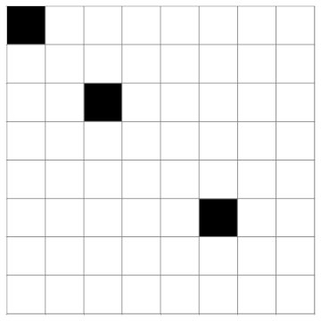
Yesterday I wrote a post about representing bit manipulations, including shifts, as matrix operators. The matrix corresponding to shifting right by k bits has 1s on the kth diagonal above the main diagonal and 0s everywhere else. For example, here is the matrix for shifting an 8-bit number right two bits. A black square represents a 1 and a white square represents a 0.

This matrix isn’t invertible. When you’d like to take the inverse of a non-invertible matrix, your knee jerk response should be to compute the pseudoinverse. (Technically the Moore-Penrose pseudoinverse. There are other pseudoinverses, but Moore-Penrose is the most common.)

As you might hope/expect, the pseudoinverse of a right-shift matrix is a left-shift matrix. In this case the pseudoinverse is simply the transpose, though of course that isn’t always the case.

If you’d like to prove that the pseudoinverse of a matrix that shifts right by k places is a matrix that shifts left by k places, you don’t have to compute the pseudo inverse per se: you can verify your guess. This post gives four requirements for a pseudoinverse. You can prove that left shift is the inverse of right shift by showing that it satisfies the four equations.

The linear algebra of bit twiddling

The previous post looked at the tempering step of the Mersenne Twister, formulating a sequence of bit operations as multiplication by a matrix mod 2. This post will look at the components more closely.

The theorems of linear algebra generally hold independent of the field of scalars. Typically the field is ℝ or ℂ, but most of basic linear algebra works the same over every field [1]. In particular, we can do linear algebra over a finite field, and we’re interested in the most finite of finite fields GF(2), the field with just two elements, 0 and 1.

In GF(2), addition corresponds to XOR. We will denote this by ⊕ to remind us that although it’s addition, it’s not the usual addition, i.e. 1 ⊕ 1 = 0. Similarly, multiplication corresponds to AND. We’ll work with 8-bit numbers to make the visuals easier to see.

Shifting a number left one bit corresponds to multiplication by a matrix with 1’s below the diagonal main. Shifting left by k bits is the same as shifting left by 1 bit k times, so the the matrix representation for x << k is the kth power of the matrix representation of shifting left once. This matrix has 1s on the kth diagonal below the main diagonal. Below is the matrix for shifting left two bits, x << k.

Right shifts are the mirror image of left shifts. Here’s the matrix for shifting right two bits, x >> k.

Shifts are not fully invertible because bits either fall off the left or the right end. The steps in the Mersenne Twister are invertible because shifts are always XOR’d with the original argument. For example, although the function that takes x to x >> 2 is not invertible, the function that takes x to x ⊕ (x >> 2) is invertible. This operation corresponds to the matrix below.

This is an upper triangular matrix, so its determinant is the product of the diagonal elements. These are all 1s, so the determinant is 1, and the matrix is invertible.

Bitwise AND multiplies each bit of the input by the corresponding bit in another number known as the mask. The bits aligned with a 1 are kept and the bits aligned with a 0 are cleared. This corresponds to multiplying by a diagonal matrix whose diagonal elements correspond to the bits in the mask. For example, here is the matrix that corresponds to taking the bitwise AND with 10100100.

Each of the steps in the Mersenne Twister tempering process are invertible because they all correspond to triangular matrices with all 1’s on the diagonal. For example, the line

y ^= (y <<  7) & 0x9d2c5680 

says to shift the bits of y left 7 places, then zero out the elements corresponding to 0s in the mask, then XOR the result with y. In matrix terms, we multiply by a lower triangular matrix with zeros on the main diagonal, then multiply by a diagonal matrix that zeros out some of the terms, then add the identity matrix. So the matrix corresponding to the line of code above is lower triangular, with all 1s on the diagonal, so it is invertible.

[1] Until you get to eigenvalues. Then it matters whether the field is algebraically complete, which no finite field is.

Unified config files

I try to maintain a consistent work environment across computers that I use. The computers differ for important reasons, but I’d rather they not differ for unimportant reasons.

Unified keys

One thing I do is remap keys so that the same key does the same thing everywhere, to the extent that’s practical. This requires remapping keys. In particular, I want the key functionality, not the key name, to be the same across operating systems. For example, the Command key on a Mac does what the Control key does on Windows and Linux. I have my machines set up so the key in the lower left corner, whatever you call it, does things like copy, paste, and cut.

Unified config files

I use bash everywhere even though zshell is the default on Mac OS. But Linux and MacOS are sufficiently different that I have two .bashrc files, one for each OS. However, both .bashrc files source a common file .bash_aliases for aliases. You can set that up by putting the following code in your .bashrc file.

if [ -f ~/.bash_aliases ]; then
    . ~/.bash_aliases
fi

Sometimes you need some kind of branching logic even for two machines running the same OS. For example, if you have two computers, named Castor and Pollux, you might have code like the following in your .bashrc.

HOSTNAME_SHORT=$(hostname -s)
if [ "$HOSTNAME_SHORT" = "Castor" ]; then
...
elif [ "$HOSTNAME_SHORT" = "Pollux" ]; then
...

One problem with using hostname is that the OS can change the name on you. At least MacOS will do this; I don’t know whether other operating systems will. If you give your machine an uncommon name then this is unlikely to happen.

I have one init.el file for Emacs. It contains some branching logic for OS:

(cond
    ((string-equal system-type "windows-nt") ; Microsoft Windows
     ...)
    ((string-equal system-type "gnu/linux") ; linux
     ...)
    ((string-equal system-type "darwin") ; Mac
     ...)
)

You can also branch on hostname.

(if (string-equal (system-name) "Castor")
...)
(if (string-equal (system-name) "Pollux")
...)

This isn’t difficult, but in the short run it’s easier to just make one ad hoc edit to a config file at a time, letting the files drift apart. Along those lines, see bicycle skills.