The length of antenna you need to receive a radio signal is proportional to the signal’s wavelength, typically 1/2 or 1/4 of the wavelength. Cell phones operate at gigahertz frequencies, and so the antennas are small enough to hide inside the phone.
But AM radio stations operate at much lower frequencies. For example, there’s a local station, KPRC, that broadcasts at 950 kHz, roughly one megahertz. That means the wavelength of their carrier is around 300 meters. An antenna as long as a quarter of a wavelength would be roughly as long as a football field, and yet people listen to AM on portable radios. How is that possible?
There are two things going on. First, transmitting is very different than receiving in terms of power, and hence in terms of the need for efficiency. People are not transmitting AM signals from portable radios.
Second, the electrical length of an antenna can be longer than its physical length, i.e. an antenna can function as if it were longer than it actually is. When you tune into a radio station, you’re not physically making your antenna longer or shorter, but you’re adjusting electronic components that make it behave as if you were making it longer or shorter. In the case of an AM radio, the electrical length is orders of magnitude more than the physical length. Electrical length and physical length are closer together for transmitting antennas.
Here’s what a friend of mine, Rick Troth, said when I asked him about AM antennas.
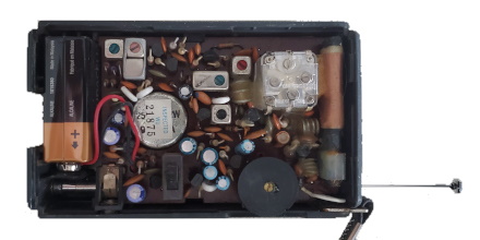
If you pop open the case of a portable AM radio, you’ll see a “loop stick”. That’s the AM antenna. (FM broadcast on most portables uses a telescoping antenna.) The loop is tuned by two things: a ferrite core and the tuning capacitor. The core makes the coiled wiring of the antenna resonate close to AM broadcast frequencies. The “multi gang” variable capacitor coupled with the coil forms an LC circuit, for finer tuning. (Other capacitors in the “gang” tune other parts of the radio.) The loop is small, but is tuned for frequencies from 530KHz to 1.7MHz.
Loops are not new. When I was a kid, I took apart so many radios. Most of the older (tube type, and AM only) radios had a loop inside the back panel. Quite different from the loop stick, but similar electrical properties.
Car antennas don’t match the wavelengths for AM broadcast. Never have. That’s a case where matching matters less for receivers. (Probably matters more for satellite frequencies because they’re so weak.) Car antennas, whether whip from decades ago or embedded in the glass, probably match FM broadcast. (About 28 inches per side of a dipole, or a 28 inch quarter wave vertical.) But again, it does matter a little less for receive than for transmit.
In the photo above, courtesy Rick, the AM antenna is the copper coil on the far right. The telescoping antenna outside the case extends to be much longer physically than the AM antenna, even though AM radio waves are two orders of magnitude longer than FM radio waves.