Yesterday I wrote two posts about finding the peaks of the sinc function. Both focused on numerical methods, the first using a contraction mapping and the second using Newton’s method. This post will focus on the locations of the peaks rather than ways of computing them.

The first post included this discussion of the peak locations.

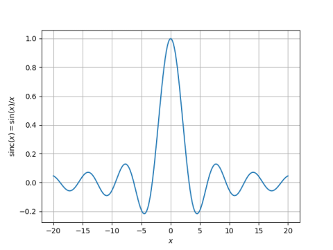
The peaks of sin(x)/x are approximately at the same positions as sin(x), and so we use (2n + 1/2)π as our initial guess. In fact, all our peaks will be a little to the left of the corresponding peak in the sine function because dividing by x pulls the peak to the left. The larger x is, the less it pulls the root over.

This post will refine the observation above. The paragraph above suggests that for large n, the nth peak is located at approximately (2n + 1/2)π. This is a zeroth order asymptotic approximation. Here we will give a first order asymptotic approximation.

For a fixed positive n, let

θ = (2n + 1/2)π

and let

x = θ + ε

be the location of the nth peak. We will improve or approximation of the location of x by estimating ε.

As described in the first post in this series, setting the derivative of the sinc function to zero says x satisfies

x cos x – sin x = 0.

Therefore

(θ + ε) cos(θ + ε) = sin(θ + ε)

Applying the sum-angle identities for sine and cosine shows

(θ + ε) (cos θ cos ε – sin θ sin ε) = sin θ cos ε + cos θ sin ε

Now sin θ = 1 and cos θ = 0, so

-(θ + ε) sin ε = cos ε.

or

tan ε = -1/(θ + ε).

So far our calculations are exact. You could, for example, solve the equation above for ε using a numerical method. But now we’re going to make a couple very simple approximations [1]. On the left, we will approximate tan ε with ε. On the right, we will approximate ε with 0. This gives us

ε ≈ -1/θ = -1/(2n + 1/2)π.

This says the nth peak is located at approximately

θ – 1/θ

where θ = (2n + 1/2)π. This refines the earlier statement “our peaks will be a little to the left of the corresponding peak in the sine function.” As n gets larger, the term we subtract off gets smaller. This makes the statement above “The larger x is, the less it pulls the root over” more precise.

Now let’s see visually how well our approximation works. The graph below plots the error in approximating the nth peak location by θ and by θ – 1/θ.

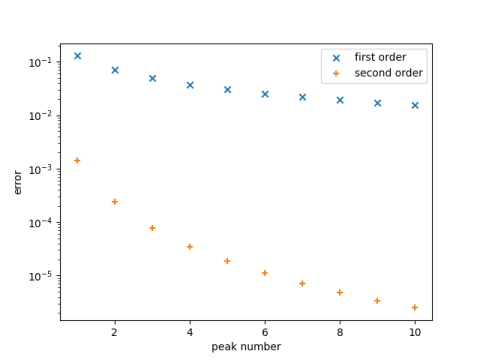
Note the log scale. The error in approximating the location of the 10th peak by 20.5π is between 0.1 and 0.01, and the error in approximating the location by 20.5π – 1/20.5π is approximately 0.000001.

[1] As pointed out in the comments, you could a slightly better approximation by not being so simple. Instead of approximating 1/(θ + ε) by 1/θ you could use 1/θ – ε/θ² and solve for ε.

In the previous post I looked at the problem of finding the peaks of the sinc function.

In this post we use this problem to illustrate how two formulations of the same problem can behave very differently with Newton’s method.

The previous post mentioned finding the peaks by solving either

x cos x – sin x = 0

or equivalently

tan x – x = 0

It turns out that the former is much better suited to Newton’s method. Newton’s method applied to the first equation will converge quickly without needing to start particularly close to the root. Newton’s method applied to the second equation will fail to converge at all unless the method beings close to the root, and even then the method may not be accurate.

Here’s why. The rate of convergence in solving

f(x) = 0

with Newton’s method is determined by the ratio of the second derivative to the first derivative

| f ‘ ‘ (x) / f ‘ (x) |

near the root.

Think of the second derivative as curvature. Dividing by the first derivative normalizes the scale. So convergence is fast when the curvature relative to the scale is small. Which makes sense intuitively: When a function is fairly straight, Newton’s method zooms down to the root. When a function is more curved, Newton’s method requires more steps.

The following table gives the absolute value of the ratio of the second derivative to the first derivative at the first ten peaks, using both equations. The bound on the error in Newton’s method is proportional to this ratio.

    |------+------------+------------|
    | peak | Equation 1 | Equation 2 |
    |------+------------+------------|
    |    1 |      0.259 |       15.7 |
    |    2 |      0.142 |       28.3 |
    |    3 |      0.098 |       40.8 |
    |    4 |      0.075 |       53.4 |
    |    5 |      0.061 |       66.0 |
    |    6 |      0.051 |       78.5 |
    |    7 |      0.044 |       91.1 |
    |    8 |      0.039 |      103.7 |
    |    9 |      0.034 |      116.2 |
    |   10 |      0.031 |      128.8 |
    |------+------------+------------|

The error terms are all small for the first equation, and they get smaller as we look at peaks further from the origin. The error terms for the second equation are all large, and get larger as we look at peaks further out.

For the third and final post in this series, see Peaks of Sinc.

Related posts

• Higher-order Newton-like methods
• Newton-Conjugate gradient method

The sinc function is defined by

sinc(x) = sin(x)/x.

This function comes up constantly in signal processing. Here’s a plot.

We would like to find the location of the function’s peaks. Let’s focus first on the first positive peak, the one that’s somewhere between 5 and 10. Once we can find that one, the rest will be easy.

If you take the derivative of sinc and set it to zero, you find that the peaks must satisfy

x cos x – sin x = 0

which means that

tan x = x.

So our task reduces to finding the fixed points of the tangent function. One way to find fixed points is simply to iterate the function. We pick a starting point near the peak we’re after, then take its tangent, then take the tangent of that, etc.

The peak appears to be located around 7.5, so we’ll use that as a starting point. Then iterates of tangent give

     2.7060138667726910
    -0.4653906051625444
    -0.5021806478408769
    -0.5491373258198057
    -0.6119188887713993
    -0.7017789436750164
    -0.8453339618848119
    -1.1276769374114777
    -2.1070512803092996
     1.6825094538261074

That didn’t work at all. That’s because tangent has derivative larger than 1, so it’s not a contraction mapping.

The iterates took us away from the root we were after. This brings up an idea: is there some way to iterate a negative number of times? Well, sorta. We can run our iteration backward.

Instead of solving

tan x = x

we could equivalently solve

arctan x = x.

Since iterating tangent pushes points away, iterating arctan should bring them closer. In fact, the derivative of arctan is less than 1, so it is a contraction mapping, and we will get a fixed point.

Let’s start again with 7.5 and iterate arctan. This quickly converges to the peak we’re after.

    7.721430101677809
    7.725188823982156
    7.725250798474231
    7.725251819823800
    7.725251836655669
    7.725251836933059
    7.725251836937630
    7.725251836937706
    7.725251836937707
    7.725251836937707

There is a little complication: we have to iterate the right inverse tangent function. Since tangent is periodic, there are infinitely many values of x that have a particular tangent value. The arctan function in NumPy returns a value between -π/2 and π/2. So if we add 2π to this value, we get values in an interval including the peak we’re after.

Here’s how we can find all the peaks. The peak at 0 is obvious, and by symmetry we only need to find the positive peaks; the nth negative peak is just the negative of the nth positive peak.

The peaks of sin(x)/x are approximately at the same positions as sin(x), and so we use (2n + 1/2)π as our initial guess. In fact, all our peaks will be a little to the left of the corresponding peak in the sine function because dividing by x pulls the peak to the left. The larger x is, the less it pulls the root over.

The following Python code will find the nth positive peak of the sinc function.

    def iterate(n, num_iterates = 6):
        x = (2*n + 0.5)*np.pi
        for _ in range(num_iterates):
            x = np.arctan(x) + 2*n*np.pi
    return x

My next post will revisit the problem in this post using Newton’s method.