Pitch of a big wine bottle

Yesterday my daughter came by and dropped off a huge blue wine bottle (empty).

Trader Joe's Incanto Chardonnay Pinot Grigio

She had started removing the label, but as you can see she didn’t get very far yet. It’s an Incanto Chardonnay Pinot Grigio from Trader Joe’s.

I blew across the top of the bottle to hear what sound it makes, and it makes a nice deep rumble.

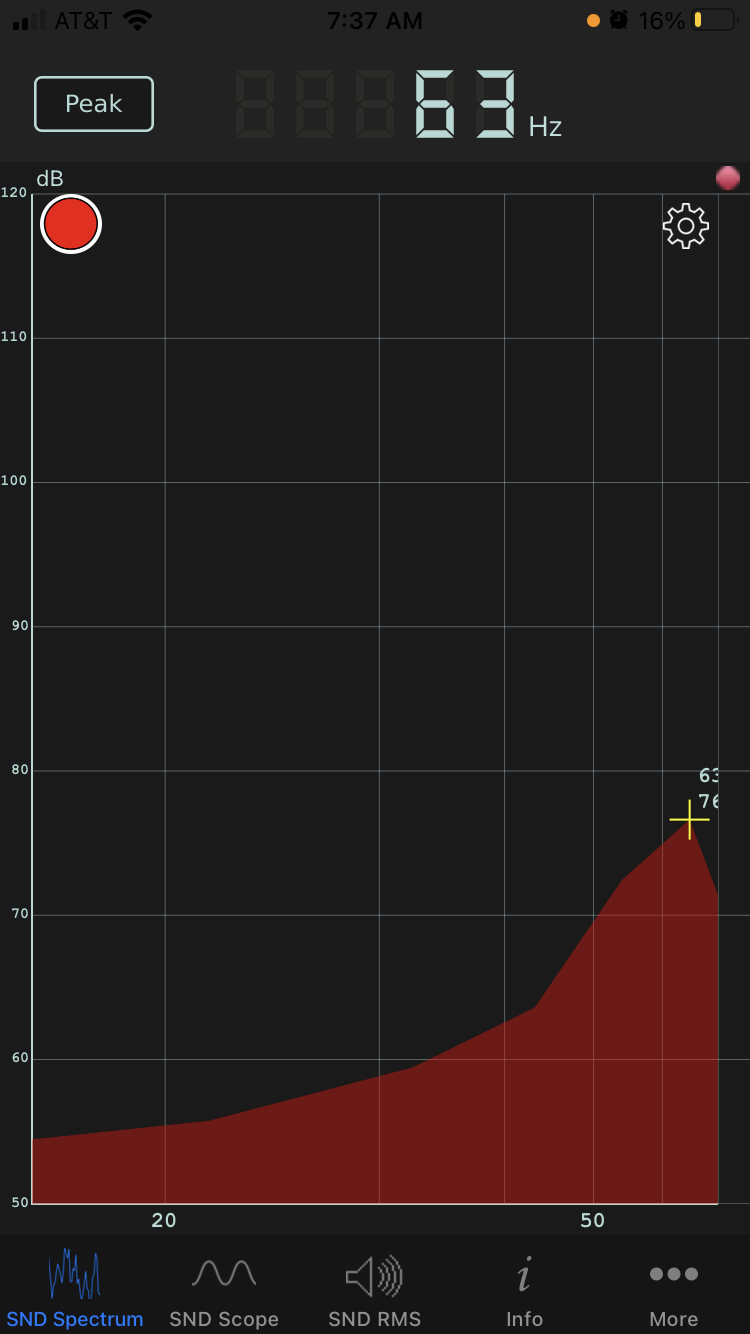
I tried to identify the pitch using a spectrum analyzer app on my phone, and it says 63 Hz.

audio spectrum analyzer screen shot

Next I tried to figure out what pitch I should expect theoretically based on physics. Wine bottles are Helmholtz resonators, and there’s a formula for the fundamental frequency of Helmholtz resonators:

f = \frac{v}{2\pi} \sqrt{\frac{A}{LV}}

The variables in this equation are:

  • f, frequency in Hz
  • v, velocity of sound
  • A, area of the opening
  • L, length of the neck
  • V, volume

I measured the opening to be 3/4 of an inch across, and the neck to be about 7 inches. The volume is 1.5 liters. The speed of sound at sea level and room temperature is 343 meters per second. After a few unit conversions [1] I got a result of 56.4 Hz, about 10% lower than what the spectrum analyzer measured.

An ideal Helmholtz resonator has a cylindrical neck attached to a spherical body. This bottle is far from spherical. The base is an ellipse with a major axis about twice as long as the minor axis. And from there it tapers off more like a cone than a sphere [2]. And yet the frequency predicted by Helmholtz’ formula comes fairly close to what I measured empirically.

I suspect I got lucky to some extent. I didn’t measure the bottle that accurately; it’s hard to even say when the neck of the bottle stops. But apparently Helmholtz’ formula is robust to changes in shape.

Update: Pitch of a beer bottle

I repeated my experiment with a beer bottle, specifically a Black Venom Imperial Stout.

Black Venom Imperial Stout

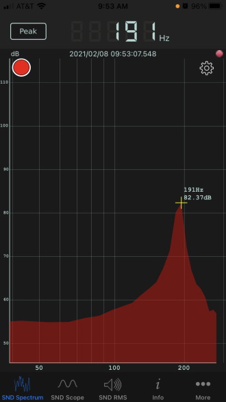
The opening diameter is about 3/4″, as with the wine bottle above, and the neck is about 3″ long. The volume is 12 fluid ounces. Helmholtz’ formula predicts a pitch of 177 Hz. My spectrum analyzer measured 191 Hz, the G below middle C. So this time theory was about 7% lower than the observed value.

Spectral analysis of blowing across beer bottle

The beer bottle is closer to the shape of a Helmholtz resonator than the wine bottle was. It’s at least radially symmetric, but the body is a cylinder rather than a sphere.

Update 2: Typical wine bottle

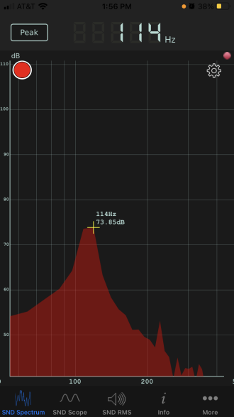
When I tested a typical 750 ml wine bottle, I got a pitch of 114 Hz. With a 3.5 inch neck and a 0.75 in diameter opening, the calculated pitch was 113 Hz. There’s some element of luck that theory and measurement agree so well, especially since the punt at the bottom means its shape is even further from spherical than that of a beer bottle.

Audio spectrum of a 750 ml pinot noir bottle

More acoustics posts

[1] Thanks to a reader who provided this write-up of the calculation:

calculation with dimensions

[2] What we usually call a cone is more specifically a right circular cone. But more generally a cone can have any base, not just a circle, and this bottle is approximately an elliptical cone.

More images from an oddball coordinate system

Three months ago I posted some images created by graphing equations in circular coordinates. Not polar coordinates as you might expect, but a strange coordinate system based on circles in another way. The most interesting thing about this coordinate system is that familiar functions product unfamiliar graphs.

This morning I played around with the code from that earlier post and made some new images.

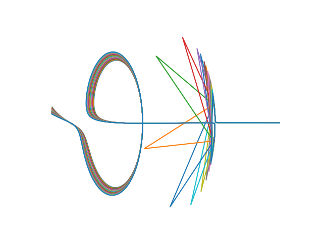
The following image was based on exp(x+7)/10 + 10*tan(x/5).

This image was based on the same function over a different range.

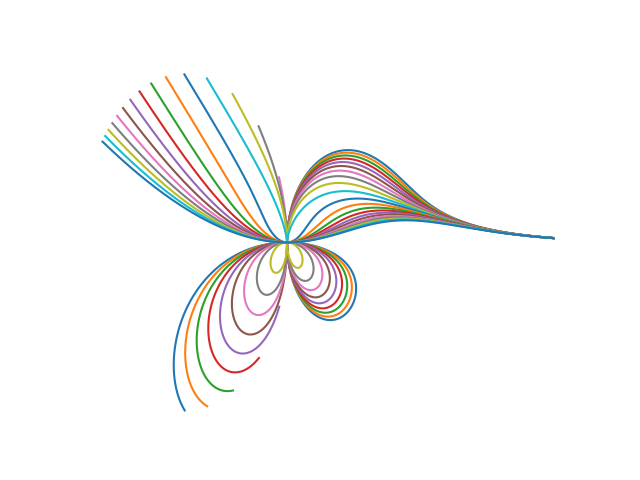
And this hummingbird-line images was based on exp(x) – x.

Here are a few more blog posts that have interesting images.

Fibonacci numbers and hyperbolic sine

Richard Askey came up with the following formula for Fibonacci numbers:

F_m = \frac{2}{\sqrt{5} \,i^m} \sinh(m \log(i\phi))

Here φ is the golden ratio, (1 + √5)/2.

We’ll use this formula as the jumping off point to discuss the implications of how equations are written, complex logarithms, and floating point computing in Python.

Reading forward and backward

Of course every equation of the form a = b can be rewritten b = a. The two forms of the equation have the same denotation but different connotations. Equations have an implied direction of application. When you see an equation written as a = b, it’s often the case that the equation is usually applied by substituting b for a.

For example, take the equation A = πr². The most natural application of this equation is that you can compute the area of a circle of radius r by squaring r and multiplying by π. It’s less common to see something like 9π and think “Oh, that’s the area of a circle of radius 3.”

Note also that this is also how nearly every programming language works: a = b means update the variable a to the value b</code.

In writing Askey’s formula as above, I’m implying that it might be useful to express the mth Fibonacci number in terms of hyperbolic sine evaluated at complex arguments. Why in the world would you want to do that? The Fibonacci numbers are elementary and concrete, but logs and hyperbolic functions are not so much, especially with complex arguments. Askey’s formula is interesting, and that would be enough, but it could be useful if some things are easier to prove using the formulation on the right side. See, for example, [1].

If I had written the formula above as

\frac{2}{\sqrt{5} \,i^m} \sinh(m \log(i\phi)) = F_m

the implication would be that the complicated expression on the left can be reduced to the simple expression on the right. It would be gratifying if some application lead naturally to the formulation on the left, but that seems highly unlikely.

I’ll close out this section with two more remarks about the direction of reading equations. First, it is a common pattern in proofs to begin by applying an equation left-to-right and to conclude by applying the same equation right-to-left. Second, it’s often a clever technique to applying an equation in the opposite of the usual order. [2]

Branch cuts

What does it mean to take the logarithm of a complex number? Well, the same as it does to take the logarithm of any number: invert the exp function. That is, log(x) = y means that y is a number such that exp(y) = x. Except that it’s not quite that simple. Notice the indefinite article: “a number such that …”. For positive real x, there is a unique real number y such that exp(y) = x. But there are infinitely many complex solutions y, even if x is real: for any integer n, exp(y + 2πni) = exp(y).

When we extend log to complex arguments, we usually want to do so in such a way that we keep familiar logs the same. We want to extend the logarithm function from the positive real axis into more of the complex plane. We can’t extend it continuously to the entire complex plane. We have to exclude some path from the origin out to infinity, and this path is known as a branch cut.

The conventional choice for log is to cut out the negative real axis. That’s what NumPy does.

Python implementation

Let’s see whether Askey’s formula works when coded up in Python.

    from numpy import sinh, log
    
    def f(m):  
        phi = (1 + 5**0.5)/2
        return 2*sinh(m*log(phi*1j))/(5**0.5*(1j)**m)

Note that Python uses j for the imaginary unit rather than i. And you can’t just use j in the code above; you have to use 1j. That let’s Python use j as an ordinary variable when it’s not part of a complex number.

When we evaluate f(1), we expect 1, the first Fibonacci number. Instead, we get

    (1-2.7383934913210137e-17j)

Although this is surprising at first glance, the imaginary part is tiny. Floating point numbers in Python have about 16 significant figures (more details here) and so the imaginary part is as close to zero as we can expect for any floating point calculation.

Here are the first five Fibonacci numbers using the code above.

    (1-2.7383934913210137e-17j)                 
    (1.0000000000000002-1.6430360947926083e-16j)
    (2-3.2860721895852156e-16j)                 
    (3.0000000000000013-7.667501775698841e-16j) 
    (5.0000000000000036-1.5061164202265582e-15j)

If you took the real part and rounded to the nearest integer, you’d have yet another program to compute Fibonacci numbers, albeit an inefficient one.

Just out of curiosity, let’s see how far we could use this formula before rounding error makes it incorrect.

    import functools

    @functools.lru_cache()
    def fib0(m):
        if m == 1 or m == 2:
            return 1
        else:
            return fib0(m-1) + fib0(m-2)

    def fib1(m):
        return round(f(m).real)

    for m in range(1, 70):
        a, b = fib0(m), fib1(m)
        if a != b:
            print(f"m: {m}, Exact: {a}, f(m): {f(m)}")

The lru_cache decorator adds memoization to our recursive Fibonacci generator. It caches computed values behind the scenes so that the code does not evaluate over and over again with the same arguments. Without it, the function starts to bog down for values of m in the 30’s. With it, the time required to execute the code isn’t noticeable.

The code above shows that fib1 falls down when m = 69.

    m: 69, Exact: 117669030460994
    f(m): (117669030460994.7-0.28813316817427764j)

Related posts

[1] Thomas Osler and Adam Hilburn. An Unusual Proof That Fm Divides Fmn Using Hyperbolic Functions. The Mathematical Gazette, Vol. 91, No. 522 (Nov., 2007), pp. 510-512.

[2] OK, a third comment. You might see equations written in different directions according to the context. For example, in a calculus book you’d see

1/(1-x) = 1 + x + x² + x³ + …

but in a book on generating functions you’re more likely to see

1 + x + x² + x³ + … = 1/(1-x)

because calculus problems start with functions and compute power series, but generating function applications create power series and then manipulate their sums. For another example, differential equation texts start with a differential equation and compute functions that satisfy the equation. Books on special functions might start with a function and then present a differential equation that the function satisfies because the latter form makes it easier to prove certain things.

Herd immunity on the back of an envelope

This post presents a back-of-the-envelope calculation regarding COVID herd immunity in the US. Every input to the calculation is only roughly known, and I’m going to make simplifying assumptions left and right. So take this all with a grain of salt.

According to a recent article, about 26 million Americans have been vaccinated against COVID, about 26 million Americans have been infected, and 1.34 million a day are being vaccinated, all as of February 1, 2021.

Somewhere around half the US population was immune to SARS-COV-2 before the pandemic began, due to immunity acquired from previous coronavirus exposure. The proportion isn’t known accurately, but has been estimated as somewhere between 40 and 60 percent.

Let’s say that as of February 1, that 184 million Americans had immunity, either through pre-existing immunity, infection, or vaccination. There is some overlap between the three categories, but we’re taking the lowest estimate of pre-existing immunity, so maybe it sorta balances out.

The vaccines are said to be 90% effective. That’s probably optimistic—treatments often don’t perform as well in the wild as they do in clinical trials—but let’s assume 90% anyway. Furthermore, let’s assume that half the people being vaccinated already have immunity, due to pre-existing immunity or infection.

Then the number of people gaining immunity each day is 0.5*0.9*1,340,000, which is about 600,000 per day. This assumes nobody develops immunity through infection from here on out, though of course some will.

There’s no consensus on how much of the population needs to have immunity before you have herd immunity, but I’ve seen numbers like 70% tossed around, so let’s say 70%.

We assumed we had 184 M with immunity on February 1, and we need 231 M (70% of a US population of 330M) to have herd immunity, so we need 47 M more people. If we’re gaining 600,000 per day through vaccination, this would take 78 days from February 1, which would be April 20.

So, the bottom line of this very crude calculation is that we should have herd immunity by the end of April.

I’ve pointed out several caveats. There are more, but I’ll only mention one, and that is that herd immunity is not an objective state. Viruses never completely go away; only one human virus—smallpox—has ever been eradicated, and that took two centuries after the development of a vaccine.

Every number in this post is arguable, and so the result should be taken with a grain of salt, as I said from the beginning. Certainly you shouldn’t put April 20 on your calendar as the day the pandemic is over. But this calculation does suggest that we should see a substantial drop in infections long before most of the population has been vaccinated.

Update: A few things have changed since this was written. For one thing, we’re vaccinating more people per day. See an update post with code you can update (or just carry out by hand) as numbers change.

More COVID posts

Pythagorean chaos

If a and b are two distinct positive integers, then

|a²-b²|,  2aba²+b²

is a Pythagorean triple. The result still gives the sides of a right triangle if the starting points aren’t integers

In [1], Nick Lord looks at what happens if you iterate this procedure, using the output of one step as the input to the next step, and look at the smaller angle of the right triangle that results.

The numbers grow exponentially, so it helps to divide a and b by c on each iteration. This prevents the series from overflowing but doesn’t change the angles.

Here’s a little Python code to explore the sequence of angles.

    import numpy as np

    θ = np.empty(50000, dtype=float)
    a, b = np.random.random(2)

    for i in range(1, N-1):
        c    = a**2 + b**2
        a, b = abs(a**2 - b**2)/c, 2*a*b/c
        θ[i] = min( np.arctan(a/b), np.arctan(b/a) )

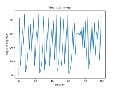
Here’s what we get if we plot the first 100 angles.

As Lord points out in [1], the series is chaotic.

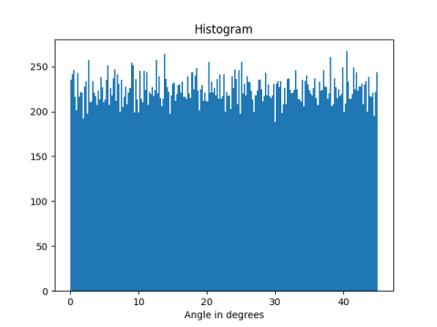
Here’s a histogram of the angles.

[1] Nick Lord. Maths bite: Pythagoras causes chaos! The Mathematical Gazette, Vol. 92, No. 524 (July 2008), pp. 290-292.

Python triple quote strings and regular expressions

There are several ways to quote strings in Python. Triple quotes let strings span multiple lines. Line breaks in your source file become line break characters in your string. A triple-quoted string in Python acts something like “here doc” in other languages.

However, Python’s indentation rules complicate matters because the indentation becomes part of the quoted string. For example, suppose you have the following code outside of a function.

x = """\
abc
def
ghi
"""

Then you move this into a function foo and change its name to y.

def foo():
    y = """\
    abc
    def
    ghi
    """

Now x and y are different strings! The former begins with a and the latter begins with four spaces. (The backslash after the opening triple quote prevents the following newline from being part of the quoted string. Otherwise x and y would begin with a newline.) The string y also has four spaces in front of def and four spaces in front of ghi. You can’t push the string contents to the left margin because that would violate Python’s formatting rules. (Update: Oh yes you can! See Aaron Meurer’s comment below.)

We now give three solutions to this problem.

Solution 1: textwrap.dedent

There is a function in the Python standard library that will strip the unwanted space out of the string y.

import textwrap 

def foo():
    y = """\
    abc
    def
    ghi
    """
    y = textwrap.dedent(y)

This works, but in my opinion a better approach is to use regular expressions [1].

Solution 2: Regular expression with a flag

We want to remove white space, and the regular expression for a white space character is \s. We want to remove one or more white spaces so we add a + on the end. But in general we don’t want to remove all white space, just white space at the beginning of a line, so we stick ^ on the front to say we want to match white space at the beginning of a line.

import re 

def foo():
    y = """\
    abc
    def
    ghi
    """
    y = re.sub("^\s+", "", y)

Unfortunately this doesn’t work. By default ^ only matches the beginning of a string, not the beginning of a line. So it will only remove the white space in front of the first line; there will still be white space in front of the following lines.

One solution is to add the flag re.MULTILINE to the substitution function. This will signal that we want ^ to match the beginning of every line in our multi-line string.

    y = re.sub("^\s+", "", y, re.MULTILINE)

Unfortunately that doesn’t quite work either! The fourth positional argument to re.sub is a count of how many substitutions to make. It defaults to 0, which actually means infinity, i.e. replace all occurrences. You could set count to 1 to replace only the first occurrence, for example. If we’re not going to specify count we have to set flags by name rather than by position, i.e. the line above should be

    y = re.sub("^\s+", "", y, flags=re.MULTILINE)

That works.

You could also abbreviate re.MULTILINE to re.M. The former is more explicit and the latter is more compact. To each his own. There’s more than one way to do it. [2]

Solution 3: Regular expression with a modifier

In my opinion, it is better to modify the regular expression itself than to pass in a flag. The modifier (?m) specifies that in the rest of the regular the ^ character should match the beginning of each line.

    y = re.sub("(?m)^\s+", "", y)

One reason I believe this is better is that moves information from a language-specific implementation of regular expressions into a regular expression syntax that is supported in many programming languages.

For example, the regular expression

    (?m)^\s+

would have the same meaning in Perl and Python. The two languages have the same way of expressing modifiers [3], but different ways of expressing flags. In Perl you paste an m on the end of a match operator to accomplish what Python does with setting flasgs=re.MULTILINE.

One of the most commonly used modifiers is (?i) to indicate that a regular expression should match in a case-insensitive manner. Perl and Python (and other languages) accept (?i) in a regular expression, but each language has its own way of adding modifiers. Perl adds an i after the match operator, and Python uses

    flags=re.IGNORECASE

or

    flags=re.I

as a function argument.

More on regular expressions

[1] Yes, I’ve heard the quip about two problems. It’s funny, but it’s not a universal law.

[2] “There’s more than one way to do it” is a mantra of Perl and contradicts The Zen of Python. I use the line here as a good-natured jab at Python. Despite its stated ideals, Python has more in common with Perl than it would like to admit and continues to adopt ideas from Perl.

[3] Python’s re module doesn’t support every regular expression modifier that Perl supports. I don’t know about Python’s regex module.

Mentally computing 3rd and 5th roots

A couple years ago I wrote about a trick for mentally computing the fifth root of an integer if you know that the number you’re starting with is the fifth power of a two-digit number.

This morning I wrote up a similar (and simpler) trick for cube roots as a thread on @AlgebraFact. You can find the Twitter thread starting here, or you could go to this page that unrolls the whole thread in one page.

Newton’s method spirals

In [1] the authors look at applying Newton’s root-finding method to the function

f(z) = zp

where p = a + bi. They show that if you start Newton’s method at z = 1, the kth iterate will be

(1 – 1/p)k.

This converges to 0 when a > 1/2, runs around in circles when a = 1/2, and diverges to infinity when a < 1/2.

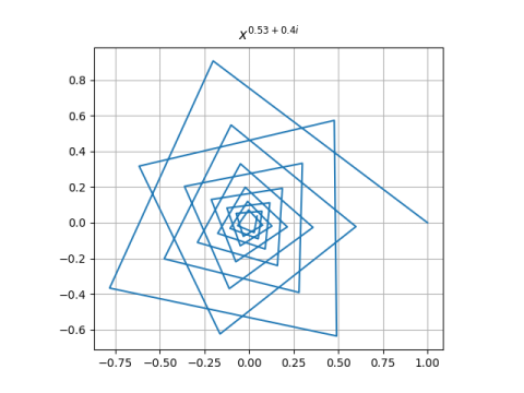
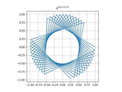
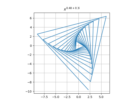
You can get a wide variety of images by plotting the iterates for various values of the exponent p. Here are three examples.

Newton's method for x^p starting at 1, p = 0.53+0.4i

Newton's method for x^p starting at 1, p = 0.5+0.3i

Newton's method for x^p starting at 1, p = 0.48+0.3i

Here’s the Python code that produced the plots.

    import numpy as np
    import matplotlib.pyplot as plt

    def make_plot(p, num_pts=40):
        k = np.arange(num_pts)
        z = (1 - 1/p)**k
        plt.plot(z.real, z.imag)
        plt.axes().set_aspect(1)
        plt.grid()
        plt.title(f"$x^{{ {p.real} + {p.imag}i }}$")
        plt.savefig(f"newton_{p.real}_{p.imag}.png")
        plt.close()

    make_plot(0.53 + 0.4j)
    make_plot(0.50 + 0.3j)
    make_plot(0.48 + 0.3j)

Note that the code uses f-strings for the title and file name. There’s nothing out of the ordinary in the file name, but the title embeds LaTeX code, and LaTeX needs its own curly braces. The way to produce a literal curly brace in an f-string is to double it.

More posts on Newton’s method

[1] Joe Latulippe and Jennifer Switkes. Sometimes Newton’s Method Always Cycles. The College Mathematics Journal, Vol. 43, No. 5, pp. 365-370

Sums of consecutive reciprocals

The sum of the reciprocals of consecutive integers is never an integer. That is, for all positive integers m and n with n > m, the sum

\sum_{k=m}^n \frac{1}{k}

is never an integer. This was proved by József Kürschák in 1908.

This means that the harmonic numbers defined by

H_n = \sum{k=1}^n \frac{1}{k}

are never integers for n > 1. The harmonic series diverges, so the sequence of harmonic numbers goes off to infinity, but it does so carefully avoiding all integers along the way.

Kürschák’s theorem says that not only are the harmonic numbers never integers, the difference of two distinct harmonic numbers is never an integer. That is, HnHm is never an integer unless m = n.

Related posts