From tape measures to tensors

tape meausre

This post will start with a motivating example, looking at measuring a room in inches and in feet. Then we will segue into a discussion of contravariance and covariance in the simplest setting. Then we will discuss contravariant and covariant tensors more generally.

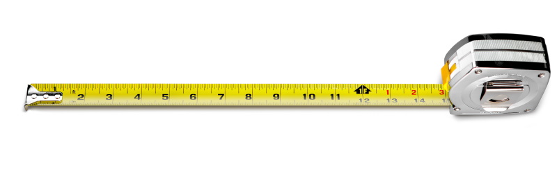
Using a tape measure

In my previous post, I explained why it doesn’t matter if a tape measure is perfectly straight when measuring a long distance. In a nutshell, if you want to measure x, but instead you measure the hypotenuse of a triangle with sides x and y, where y is much smaller than x, the difference is approximately y²/2x. The error is nowhere as big as y.

In that post I gave the example of measuring a wall that is 10 feet long, and measuring to a point 4 inches up the adjacent wall rather than measuring to the corner. The error is about 1/15 of an inch.

Now suppose we’re off by more, measuring 12 inches up the other wall. Now that we have an even foot, we can switch over to feet and work with smaller, simpler numbers. Now we have x = 10 and y = 1. So the error is approximately 1/20.

Before, we were working in inches. We had x = 120, y = 4, and error 1/15. Does that mean our error is now smaller? That can’t be. If the short leg of our triangle is longer, 12 inches rather than 4 inches, our error should go up, not down.

Of course the resolution is that our error was 1/15 of an inch in the first example, and 1/20 of a foot in the second example. If we were to redo our second example in inches, we’d get error 12²/240 = 12/20, i.e. we’d convert 1/20 of a foot to 12/20 of an inch.

Change of units and contravariance

Now here’s where tensors come in. Notice that when we use a larger unit of measurement, a foot instead of an inch, we get a smaller numerical value for error. Trivial, right? If you first measure a distance in meters, you’ll get larger numbers if you switch to centimeters, but smaller numbers if you switch to light years.

But this simple observation is an example of a deeper pattern. Measurements of this kind are contravariant, meaning that our numerical values change in the opposite direction as our units of measurement.

A velocity vector is contravariant because if you use smaller units of length, you get larger numerical values of velocity, and vice versa. Under a change of units, velocity changes in the opposite direction of the units.

A gradient vector is covariant because if you use smaller units of length, a function will vary less per unit length. Gradients change in the same direction as your units.

The discussion so far has been informal and limited to a very special change of coordinates. It’s not just the direction of change that matters, that results change monotonically with units, but that they increase or decrease by the exact same proportion. And the kinds of coordinate changes we usually have in mind are not changing from inches to feet but rather changing from rectangular coordinates to polar coordinates.

More general and more formal

Suppose you have some function T described by coordinates denoted by x‘s with superscripts. Put bars on top of everything to denote a new representation of T with respect to new coordinates. If T is a contravariant vector we have,

\bar{T}^i =T^r \frac{\partial \bar{x}^i}{\partial x^r}

and if T is a covariant vector we have

\bar{T}_i =T_r \frac{\partial x^r}{\partial \bar{x}^i}

In the equations above there is an implicit summation over the repeated index r, using the so-called Einstein summation convention.

The examples at the end of the previous section are the canonical examples: tangent vectors are contravariant and gradients are covariant.

If the xs without bars are measured in inches and the xs with bars are measured in feet, the partial derivative of an x bar with respect to the corresponding x is 1/12, because a unit change in inches causes a change of 1/12 in feet.

Vectors are a special case of tensors, called 1-tensors. Higher order tensors satisfy analogous rules. A 2-tensor is contravariant if

 \bar{T}^{ij} = T^{rs} \frac{\partial\bar{x}^i}{\partial x^r} \frac{\partial\bar{x}^j}{\partial x^s}

and covariant if

\bar{T}_{ij} = T_{rs} \frac{\partial x^r}{\partial\bar{x}^i} \frac{\partial x^s}{\partial \bar{x}^j}

Even more generally you can have tensors of any order, and they can be contravariant in some components and covariant in others.

Backing up

For more on tensors, you may want to read a five-part series of blog posts I wrote starting with What is a tensor?. The word “tensor” is used in several related but different ways. The view of tensors given here, as things that transform a certain way under changes of coordinates, is discussed in the fourth post in that series.

It doesn’t matter much if the tape is straight

Architect measureing floor

Suppose a contractor is measuring the length of a wall. He starts in one corner of the room, and lets out a tape measure heading for the other end of the wall. But something is in the way, so instead of measuring straight to the corner, he measures to a point near the corner on the adjacent wall.

If you looked down on the room from a bird’s eye view, the contractor wants to measure the distance from (0, 0) to (x, 0), but instead measures from (0, 0) to (x, y) where y is small relative to x. How much difference does this make?

The measurement error, as a function of y, is given by

(x² + y²)1/2x.

Expanding this function in a Taylor series around y = 0 shows that the error is approximately

y²/2x.

So the error is not on the order of y but of y²/x. The latter is much smaller if y is small relative to x.

For example, suppose a room is 10 feet (120 inches) long. If someone were to measure the length of the room by running a tape measure to a point 4 inches up the joining wall, the measurement error would not be anywhere near 4 inches but rather nearly 16/240 = 1/15 of an inch.

Let’s work this example out and see how good the approximation was. The hypotenuse of a right triangle with sides 120 and 4 is

√14416 = 120.066648…

which is very close to

120 + 1/15 = 120.06666…

The fact that the measurement wasn’t exactly corner-to-corner would likely not be the largest source of measurement error.

Update: What if the measuring tape sags in the middle?

At the next prime, turn left

The previous post mentioned a Math Overflow question about unexpected mathematical images, and reproduced one that looks like field grass. This post reproduces another set of images from that post.

Start anywhere in the complex plane with integer coordinates and walk west one unit at a time until you run into Gaussian prime [1]. Then turn left (counterclockwise) 90° and keep taking unit steps. Apparently this process will often (always?) return you to your starting point.

Different starting points lead to different patterns. Here’s an example given in the post, starting at 3 + 5i.

starting at 3 + 5i

Here’s a more complex walk starting at 27 + 30i.

starting at 3 + 5i

I tried starting at 127 + 131i and got a simple, uninteresting image. I tried again starting at 127 + 130i and got something much more complicated. I didn’t time it, but it took several minutes to plot.

starting at 3 + 5i

Here’s the code that made the plots. (Note that Python uses j rather than i for imaginary unit.)

Update: The code below originally set the aspect ratio using

plt.axes().set_aspect(1)

Apparently matplotlib has changed since the code was written, and the original code produces strange results. The line of code

plt.gca().set_aspect("equal")

works now (April 27, 2024).

from sympy import isprime
import matplotlib.pyplot as plt

def isgaussprime(z: complex):
    a, b = int(z.real), int(z.imag)
    if a*b != 0:
        return isprime(a**2 + b**2)
    else:
        c = abs(a+b)
        return isprime(c) and c % 4 == 3

def connect(z1: complex, z2: complex):
    plt.plot([z1.real, z2.real], [z1.imag, z2.imag], 'b')
    
start = 127 + 130j
#start = 3 + 5j
step = 1
z = start
next = None

while next != start:
    next = z + step
    connect(z, next)
    if isgaussprime(next):
        step *= 1j
    z = next

plt.gca().set_aspect("equal")    
plt.show()

Related posts

[1] If a and b are integers, then a + bi is called a Gaussian integer. A Gaussian integer is a Gaussian prime if (1) both a and b are non-zero and a² + b² is prime, or (2) one of a or b is zero, and the absolute value of the non-zero part is a prime congruent to 3 mod 4.

Why is this definition so complicated? It’s actually a theorem. There’s a natural generalization of what it means to be prime in a commutative ring, and it works out that an element the Gaussian integers is prime if and only if the above criteria hold.

In general, a non-zero element p of a commutative ring R is prime if whenever p divides a product ab, p must either divide a or divide b.

Simple equations whose plot looks like field grass

Math Overflow has an interesting question about unexpected mathematical images. Here’s a response from Payam Seraji that was easy to code up.

Here’s the code that produced the image.

from numpy import *
import matplotlib.pyplot as plt

t = linspace(0, 39*pi/2, 1000)
x = t*cos(t)**3
y = 9*t*sqrt(abs(cos(t))) + t*sin(0.2*t)*cos(4*t)
plt.plot(x, y, c="green")
plt.axes().set_aspect(0.3)
plt.axis('off')

Constructing bilinear transformations

The previous post was a visual introduction to bilinear transformations, a.k.a. Möbius transformations or fractional linear transformations. This post is a short follow-up focused more on calculation.

A bilinear transformation f has the form

f(z) = \frac{az + b}{cz + d}

where adbc ≠ 0.

Inverse

The inverse of f is given by

 g(w) = \frac{dw - b}{-cw + a}

The transformation f is defined everywhere except at z = –d/c, and its inverse is defined everywhere except at w = a/c.

So f takes the complex plane minus one point to the complex plane minus one point. Or an elegant way of thinking about it is to think of f and g as functions on a sphere by adding a point at infinity. Then we say

\begin{align*} f(-d/c) &= \infty \\ g(\infty) &= -d/c \\ f(\infty) = a/c \\ g(a/c) &= \infty \end{align*}

Determining by three points

Bilinear transformations have three degrees of freedom. That is, you can pick three values in the domain and specify three places for them to go in the range. The unique bilinear transform sending z1, z2, and z3 to w1, w2, and w3 is given by

\frac{(w - w_2)(w_3 - w_1)}{(w - w_1)(w_3 - w_2)} = \frac{(z - z_2)(z_3 - z_1)}{(z - z_1)(z_3 - z_2)}

Plug in your constants and solve for w = f(z).

Update: Here are explicit formulas for the coefficients.

Example

For example, let’s look at the smiley face example from the previous post.

We’ll pick three points on the face and three places for them to go.

Let’s say we want the center of the face to stay put, mapping 0 to 0. Next let’s pick two places for the center of the eyes to go. These are at
±0.4+.2ji. Say we want the left eye to go down a little to -0.4 and the right eye to go up and over a little to 0.5 + 0.3i.

I used Mathematica to solve for the parameters.

    {z1, z2, z3} = {0, -2/5 + I/5, 2/5 + I/5}
    {w1, w2, w3} = {0, -2/5, 1/2 + 3 I/10}
    Solve[(w - w2) (w3 - w1)/((w - w1) (w3 - w2)) == 
          (z - z2) (z3 - z1)/((z - z1) (z3 - z2)), w]

This says the parameters are, in Python notation,

    a = -72 - 16j
    b = 0
    c = 30 - 35j
    d = -75

Using the code from the previous post we can verify that this transformation does what we designed it to do.

    print(mobius(0, a, b, c, d))
    print(mobius(-0.4 + 0.2j, a, b, c, d))
    print(mobius(0.4 + 0.2j, a, b, c, d))

and we can take a look at the result.

Related posts

Circles to Circles

This post expands on something I said in passing yesterday. I said in the body of the post that

… the image of a circle in the complex plane under a Möbius transformation is another circle.

and added in a footnote that

For this to always be true, you have to include a line as a special case of a circle, a circle of infinite radius if you like.

This post will illustrate these statements with Python code and plots. First, some code for drawing circles and other curves in the complex plane.

    from numpy import exp, pi, linspace
    import matplotlib.pyplot as plt

    θ = linspace(0, 2*pi, 200)

    def circle(radius, center):
        return center + radius*exp(1j*θ)

    def plot_curves(curves):
        for c in curves:
            plt.plot(c.real, c.imag)
        plt.axes().set_aspect(1)
        plt.show()
        plt.close()

Next, code for Möbius transformations, and the particular Möbius transformation we’ll use in our plots.

    def mobius(z, a, b, c, d):
        return (a*z + b)/(c*z + d)

    def m(curve):
        return mobius(curve, 1, 2, 3, 4)

Now we’ll plot three circles and their images under the Möbius transformation

m(z) = (z + 2)/(3z + 4)

with the following code.

    circles = [circle(1, 0), circle(2, 0), circle(2, 2)]
    plot_curves(circles)
    plot_curves([m(c) for c in circles])

This produces

and

Notice that the first circle, in blue, started out as the smallest circle and was contained inside the second circle, in orange. But in the image, the blue circle became the largest, and is no longer inside the orange circle. That is because our Möbius transformation has a singularity at -4/3, and things get turned inside-out around that point.

Next we’ll look at an example of lines being mapped to lines.

    line = linspace(-100, 100, 600)
    curves = [line, 1j*line - 4/3]
    plot_curves(curves)
    plot_curves([m(c) for c in curves])

This produces

and

These lines are mapped to lines because they both pass through the singularity at -4/3. The real axis, in blue, is mapped to itself. The line -4/3 + iy, is shifted over to have real part 1/3.

Finally, lets look at lines being mapped to circles. Since the inverse of a Möbius transformation is another Möbius transformation, this example also shows that circles can be mapped to lines.

    
    lines = [1j*line - 4, 1j*line + 4, line - 4j, line + 4j]
    plot_curves(lines)
    plot_curves([m(c) for c in lines])

This produces

and

Note that the circles don’t quite close. That’s because my line only runs from -100 to 100, not -∞ to ∞. The gap in the circles is at 1/3, because that’s the limit of our transformation (z + 2)/(3z + 4) as z goes to ±∞.

Smiley faces

To illustrate things further, I’d like to look at a smiley face and what happens to it under different Möbius transformations.

Here’s the code to draw the original face.

    dash = linspace(0.60, 0.90, 20)
    smile = 0.3*exp(1j*2*pi*dash) - 0.2j
    left_eye  = circle(0.1, -0.4+.2j)
    right_eye = circle(0.1,  0.4+.2j)
    face = [circle(1, 0), left_eye, smile, right_eye]

Next, let’s subject this face to the Möbius transformation with parameters (1, 0, 1, 3). The singularity is at -3, outside the face and fairly far away.

Next we’ll use parameters (1, 0, 1, -1+1j), which has a sigularity at 1 – i, closer to the face, and hence more distortion.

Now we use parameters (1, 0, 3, 1), putting the singularity at -1/3, inside the face.

Finally, we look at parameters (1, 0, 1, 0.4-0.2j), putting the singularity inside the left eye.

The next post explains how to pick the parameters of a Möbius transformation to make points go where you want.

Simultaneous projects

I said something to my wife this evening to the effect that it’s best for employees to have one or at most two projects at a time. Two is good because you can switch off when you’re tired of one project or if you’re waiting on input. But with three or more projects you spend a lot of time task switching.

She said “But …” and I immediately knew what she was thinking. I have a lot more than two projects going on. In fact, I would have to look at my project tracker to know exactly how many projects I have going on right now. How does this reconcile with my statement that two projects is optimal?

Unless you’re doing staff augmentation contracting, consulting work is substantially different from salaried work. For one thing, projects tend to be smaller and better defined.

Also consultants, at least in my experience, spend a lot of time waiting on clients, especially when the clients are lawyers. So you take on more work than you could handle if everyone wanted your attention at once. At least you work up to that if you can. You balance the risk of being overwhelmed against the risk of not having enough work to do.

Working for several clients in a single day is exhausting, but that’s usually not necessary. My ideal is to do work for one or two clients each day, even if I have a lot of clients who are somewhere between initial proposal and final invoice.

Schwarzian derivative

There are many ways the basic derivative can be generalized: partial derivatives, directional derivatives, covariant derivatives, etc. These all reduce to the basic derivative under the right circumstances.

The Schwarzian derivative is not like that. It’s not a generalization of the familiar derivative but rather a differential operator analogous to a derivative. The Schwarzian derivative of a function f is defined [1] as

S(f) = \left(\frac{f''}{f'}\right)' - \frac{1}{2} \left(\frac{f''}{f'}\right)^2

To understand the motivation behind such an arbitrary-looking definition, we need to first look at functions of the form

g(z) = \frac{az + b}{cz + d}

called Möbius transformations, or more descriptively, fractional linear transformations [2]. These transformations are very important in complex analysis and have a lot of interesting properties. For example, the image of a circle in the complex plane under a Möbius transformation is another circle [3].

Möbius transformations are to the Schwarzian derivative roughly what constants are to the ordinary derivative. A function is a Möbius transformation if and only if its Schwarzian derivative is zero.

Since the Schwarzian derivative is defined in terms of ordinary derivatives, adding a constant to a function doesn’t change its Schwarzian derivative. Furthermore, the Schwarzian derivative is defined in terms of the ratio of ordinary derivatives, so multiplying a function by a constant doesn’t change its Schwarzian derivative either.

Even more generally, applying a Möbius transformation to a function doesn’t change its Schwarzian derivative. That is, for a fractional linear transformation like g(z) above

S(g \circ f) = S(f)

for any function f. So you can pull Möbius transformations out of a Schwarzian derivative sorta like the way you can pull constants out of an ordinary derivative. The difference though is that instead of the Möbius transformation moving to the outside, it simply disappears.

You can think of the Schwarzian derivative as measuring how well a function can be approximated by a Möbius transformation. Schwarzian derivatives come up frequently in applications of complex analysis, such as conformal mapping.

More kinds of derivatives

[1] The Schwarzian derivative of a constant function is defined to be zero.

[2] Möbius transformations require adbc to not equal zero.

[3] For this to always be true, you have to include a line as a special case of a circle, a circle of infinite radius if you like. If you don’t like that definition, then you can rephrase the statement above as saying Möbius transformations map circles and lines to circles and lines.

Searching Greek and Hebrew with regular expressions

According to the Python Cookbook, “Mixing Unicode and regular expressions is often a good way to make your head explode.” It is thus with fear and trembling that I dip my toe into using Unicode with Greek and Hebrew.

I heard recently that there are anomalies in the Hebrew Bible where the final form of a letter is deliberately used in the middle of a word. That made me think about searching for such anomalies with regular expressions. I’ll come back to that shortly, but I’ll start by looking at Greek where things are a little simpler.

Greek

Only one letter in Greek has a variant form at the end of a word. Sigma is written ς at the end of a word and σ everywhere else. The following Python code shows we can search for sigmas and final sigmas in the first sentence from Matthew’s gospel.

    import re

    matthew = "Κατάλογος του γένους του Ιησού Χριστού, γιου του Δαυείδ, γιου του Αβραάμ"
    matches = re.findall(r"\w+ς\b", matthew)
    print("Words ending in sigma:", matches)

    matches = re.findall(r"\w*σ\w+", matthew)
    print("Words with non-final sigmas:", matches)

This prints

    Words ending in sigma: ['Κατάλογος', 'γένους']
    Words with non-final sigmas: ['Ιησού', 'Χριστού']

This shows that we can use non-ASCII characters in regular expressions, at least if they’re Greek letters, and that the metacharacters \w (word character) and \b (word boundary) work as we would hope.

Hebrew

Now for the motivating example. Isaiah 9:6 contains the word “לםרבה” with the second letter (second from right) being the final form of Mem, ם, sometimes called “closed Mem” because the form of the letter ordinarily used in the middle of a word, מ, is not a closed curve [1].

Here’s code to show we could find this anomaly with regular expressions.

    # There are five Hebrew letters with special final forms.
    finalforms = "\u05da\u05dd\u05df\u05e3\u05e5" # ךםןףץ

    lemarbeh = "\u05dc\u05dd\u05e8\u05d1\u05d4" # לםרבה
    m = re.search(r"\w*[" + finalforms + "\w+", lemarbeh)
    if m:
        print("Anomaly found:", m.group(0))

As far as I know, the instance discussed above is the only one where a final letter appears in the middle of a word. And as far as I know, there are no instances of a non-final form being used at the end of a word. For the next example, we will put non-final forms at the end of words so we can find them.

We’ll need a list of non-final forms. Notice that the Unicode value for each non-final form is 1 greater than the corresponding final form. It’s surprising that the final forms come before the non-final forms in numerical (Unicode) order, but that’s how it is. The same is true in Greek: final sigma is U+03c2 and sigma is U+03c3.

    finalforms = "\u05da\u05dd\u05df\u05e3\u05e5" # ךםןףץ
    nonfinal   = "\u05db\u05de\u05e0\u05e4\u05e6" # כמנפצ

We’ll start by taking the first line of Genesis

    genesis = "בראשית ברא אלהים את השמים ואת הארץ"

and introduce errors by replacing each final form with its corresponding non-final form. The code uses a somewhat obscure feature of Python and is analogous to the shell utility tr.

    genesis_wrong = genesis.translate(str.maketrans(finalforms, nonfinal))

(The string method translate does what you would expect, except that it takes a translation table rather than a pair of strings as its argument. The maketrans method creates a translation table from two strings.)

Now we can find our errors.

    anomalies = re.findall(r"\w+[" + nonfinal + r"]\b", genesis_wrong)
    print("Anomalies:", anomalies)

This produced

    Anomalies: ['אלהימ', 'השמימ', 'הארצ']

Note that Python printed the letters left-to-right.

Vowel points

The text above did not contain vowel points. If the text does contain vowel points, these are treated as letters between the consonants.

For example, the regular expression “בר” will not match against “בְּרֵאשִׁית” because the regex engine sees two characters between ב and ר, the dot (“dagesh”) inside ב and the two dots (“sheva”) underneath ב. But the regular expression “ב..ר” does match against “בְּרֵאשִׁית”.

See footnote [1].

Python

I started this post with a warning from the Python Cookbook that mixing regular expressions and Unicode can cause your head to explode. So far my head intact, but I’ve only tested the waters. I’m sure there are dragons in the deeper end.

I should include the rest of the book’s warning. I used the default library re that ships with Python, but the authors recommend if you’re serious about using regular expressions with Unicode,

… you should consider installing the third-party regex library which provides full support for Unicode case folding, as well as a variety of other interesting features, including approximate matching.

Related posts

[1] When I refer to “בר” as a regular expression, I mean the character sequence ב followed by ר, which your browser will display from right to left because it detects it as characters from a language written from right to left. Written in terms of Unicode code points this would be “\u05d1\u05e8”, the code point for ב followed by the code point for ר.

Similarly, the second regular expression could be written “\u05d1..\u05e8”. The two periods in the middle are just two instances of the regular expression symbol that matches any character. It’s a coincidence that dots (periods) are being used to match dots (the dagesh and the sheva).

Descartes and Toolz

I was looking recently at the Python module toolz, a collection of convenience functions. A lot of these functions don’t do that much. They don’t save you much code, but they do make your code more readable by making it more declarative. You may not realize need them until you see them.

For example, there is a function partitionby that breaks up a sequence at the points where a given function’s value changes. I’m pretty sure that function would have improved some code I’ve written recently, making it more declarative than procedural, but I can’t remember what that was.

Although I can’t think of my previous example, I can think of a new one, and that is Descartes’ rule of signs.

Given a polynomial p(x), read the non-zero coefficients in order and keep note of how many times they change sign, either from positive to negative or vice versa. Call that number n. Then the number of positive roots of p(x) either equals n or n minus a positive even number.

For example, suppose

p(x) = 4x4 + 3.1x3x2 – 2x + 6.

The coefficients are 4, 3.1, -1, -2, and 6. The list of coefficients changes signs twice: from positive to negative, and from negative to positive. Here’s a first pass at how you might have Python split the coefficients to look sign changes.

    from toolz import partitionby

    coefficients = [4, 3.1, -1, -2, 6]
    parts = partitionby(lambda x: x > 0, coefficients)
    print([p for p in parts])

This prints

    [(4, 3.1), (-1, -2), (6,)]

The first argument to partitionby an anonymous function that tests whether its argument is positive. When this function changes value, we have a sign alteration. There are three groups of consecutive coefficients that have the same sign, so there are two times the signs change. So our polynomial either has two positive roots or no positive roots. (It turns out there are no positive roots.)

The code above isn’t quite right though, because Descartes said to only look at non-zero coefficients. If we change our anonymous function to

    lambda x: x >= 0

that will work for zeros in the middle of positive coefficients, but it will give a false positive for zeros in the middle of negative coefficients. We can fix the code with a list comprehension. The following example works correctly.

    coefficients = [4, 0, 3.1, -1, 0, -2, 6]
    nonzero = [c for c in coefficients if c != 0]
    parts = partitionby(lambda x: x > 0, nonzero)
    print([p for p in parts])

If our coefficients were in a NumPy array rather than a list, we could remove the zeros more succinctly.

    from numpy import array

    c = array(coefficients)
    parts = partitionby(lambda x: x > 0, c[c != 0])

The function partitionby returns an iterator rather than a list. That’s why we don’t just print parts above. Instead we print [p for p in parts] which makes a list. In applications, it’s often more efficient to have an iterator than a list, generating items if and when they are needed. If you don’t need all the items, you don’t have to generate them all. And even if you do need all the items, you could save memory by not keeping them all in memory at once. I’ll ignore such efficiencies here.

We don’t need the partitions per se, we just need to know how many there are. The example that escapes my mind would have been a better illustration if it needed to do more with each portion than just count it. We could count the number of sign alternations for Descartes rule as follows.

   len([p for p in parts]) - 1

Related posts