Solving hard problems

We help companies solve hard problems in mathematics, statistics, and computing. Let’s explore how we might work together.

Sine series for a sine

Posted on 7 April 2020 by John

The Fourier series of an odd function only has sine terms—all the cosine coefficients are zero—and so the Fourier series is a sine series.

What is the sine series for a sine function? If the frequency is an integer, then the sine series is just the function itself. For example, the sine series for sin(5x) is just sin(5x). But what if the frequency is not an integer?

For an odd function f on [-π, π] we have

$f(x) = \sum_{n=0}^\infty c_n \sin(n x)$

where the coefficients are given by

$c_n = \frac{1}{\pi} \int_{-\pi}^\pi f(x) \sin(nx)\, dx$

So if λ is not an integer, the sine series coefficients for sin(λx) are given by

$c_n = 2\sin(\lambda \pi) (-1)^n \,\frac{ n}{\pi(\lambda^2 - n^2)}$

The series converges slowly since the coefficients are O(1/n).

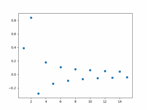
For example, here are the first 15 coefficients for the sine series for sin(1.6x).

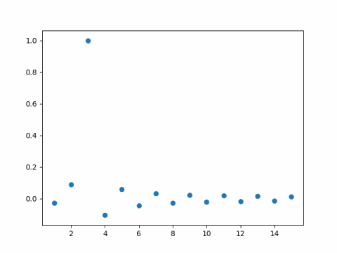
And here is the corresponding plot for sin(2.9x).

As you might expect, the coefficient of sin(3x) is nearly 1, because 2.9 is nearly 3. What you might not expect is that the remaining coefficients are fairly large.

Update: After writing this post I wrote another on the rate of convergence for Fourier series. In general, the smoother the function, the faster the Fourier series converges and vice versa, with some fine print.

The sine function above is perfectly smooth, but it’s Fourier series converges slowly. How can that be? The Fourier series is defined for periodic functions. If k is not an integer and we force sin(kx) to be a function with period 2π, it is not continuous. When we extend sin(kx) to make it periodic, there’s a jump discontinuity at the ends of each period.

Look back at

$f(x) = \sum_{n=0}^\infty c_n \sin(n x)$

This equation can’t hold everywhere. If k is not an integer and f(x) = sin(kx), then the right size is zero at π but the left is not. In fact we’ll see Gibbs phenomenon at π because of the discontinuity there.

Two meanings of QR code

Posted on 7 April 2020 by John

“QR code” can mean a couple different things. There is a connection between these two, though that’s not at all obvious.

What almost everyone thinks of as a QR code is a quick response code, a grid of black and white squares that encode some data. For example, the QR code below contains my contact info.

There’s also something in algebraic coding theory called a QR code, a quadratic residue code. These are error-correcting codes that are related to whether numbers are squares or not modulo a prime.

The connection between quick response codes and quadratic residue codes is that both involve error-correcting codes. However, quick response codes use Reed-Solomon codes for error correction, not quadratic residue codes. Reed-Solomon codes are robust to long sequences of error, which is important for quick response codes since, for example, a row of the image might be cut off. It would be cute if QR (quick response) codes used QR (quadratic residue) codes, but alas they don’t.

Center of mass and vectorization

Posted on 5 April 2020 by John

Para Parasolian left a comment on my post about computing the area of a polygon, suggesting that I “say something similar about computing the centroid of a polygon using a similar formula.” This post will do that, and at the same time discuss vectorization.

Notation

We start by listing the vertices starting anywhere and moving counterclockwise around the polygon:

$(x_1, y_1), (x_2, y_2), \cdots, (x_n, y_n)$

It will simplify notation below if we duplicate the last point:

The formula the centroid depends on the formula for the area, where the area of the polygon is

$A = \frac{1}{2} \sum_{i=0}^{n-1} (x_i y_{i+1} - x_{i+1}y_i)$

Hadamard product and dot product

We can express the area formula more compactly using vector notation. This will simplify the centroid formulas as well. To do so we need to define two ways of multiplying vectors: the Hadamard product and the dot product.

The Hadamard product of two vectors is just their componentwise product. This is a common operation in R or Python, but less common in formal mathematics. The dot product is the sum of the components of the Hadamard product.

If x and y are vectors, the notation xy with no further explanation probably means the dot product of x or y if you’re reading a math or physics book. In R or Python, x*y is the Hadamard product of the vectors.

Here we will use a circle ∘ for Hadamard product and a dot · for inner product.

Now let x with no subscript be the vector

$x = (x_0, x_1, x_2, \cdots, x_{n-1})$

and let x‘ be the same vector but shifted

$x' = (x_1, x_2, x_3, \cdots, x_n)$

We define y and y‘ analogously. Then the area is

$A = (x\cdot y' - x' \cdot y) / 2$

Centroid formula

The formula for the centroid in summation form is

$\begin{align*} C_x &= \frac{1}{6A} \sum_{i=0}^{n-1} (x_i + x_{i+1})(x_i y_{i+1} - x_{i+1}y_i) \\ C_y &= \frac{1}{6A} \sum_{i=0}^{n-1} (y_i + y_{i+1})(x_i y_{i+1} - x_{i+1}y_i) \end{align*}$

where A is the area given above.

We can write this in vector form as

$\begin{align*} C_x &= \frac{1}{6A} (x + x') \cdot (x\circ y' - x' \circ y) \\ C_y &= \frac{1}{6A} (y + y') \cdot (x\circ y' - x' \circ y) \\ \end{align*}$

You could evaluate v = x∘ y‘ – x‘∘y first. Then A is half the dot product of v with a vector of all 1’s, and the centroid x and y coordinates are inner products of v with x + x‘ and y + y‘ respectively, divided by 6A.

Making an invertible function out of non-invertible parts

Posted on 4 April 2020 by John

How can you make an invertible function out of non-invertable parts? Why would you want to?

Encryption functions must be invertible. If the intended recipient can’t decrypt the message then the encryption method is useless.

Of course you want an encryption function to be really hard to invert without the key. It’s hard to think all at once of a function that’s really hard to invert. It’s easier to think of small components that are kinda hard to invert. Ideally you can iterate steps that are kinda hard to invert and create a composite that’s really hard to invert.

So how do we come up with components that are kinda hard to invert? One way is to make small components that are non-linear, and that are in fact impossible to invert [1]. But how can you use functions that are impossible to invert to create functions that are possible to invert? It doesn’t seem like this could be done, but it can. Feistel networks, named after cryptographer Horst Feistel, provide a framework for doing just that.

Many block encryption schemes are based a Feistel network or a modified Feistel network: DES, Lucifer, GOST, Blowfish, LOKI, etc.

The basic idea of Feistel networks is so simple that it may go by too fast the first time you see it.

You take a block of an even number bits and split it into two sub-blocks, the left half L and the right half R. The nth round of a Feistel cipher creates new left and right blocks from the left and right blocks of the previous round by

$\begin{align*} L_n =& R_{n-1} \\ R_n =& L_{n-1} \oplus f(R_{n-1}, K_n) \end{align*}$

Here ⊕ is bitwise XOR (exclusive or) and f(R_n-1, K_n) is any function of the previous right sub-block and the key for the nth round. The function f need not be invertible. It could be a hash function. It could even be a constant, crushing all input down to a single value. It is one of the non-invertible parts that the system is made of.

Why is this invertible? Suppose you have L_n and R_n. How could you recover L_n-1 and R_n-1?

Recovering R_n-1 is trivial: it’s just L_n. How do you recover L_n-1? You know R_n-1 and the key K_n and so you can compute

$R_n \oplus f(R_{n-1}, K_n) = L_{n-1} \oplus f(R_{n-1}, K_n)\oplus f(R_{n-1}, K_n) = L_{n-1}$

The main idea is that XOR is its own inverse. No matter what f(R_n-1, K_n) is, if you XOR it with anything twice, you get that thing back.

At each round, only one sub-block from the previous round is encrypted. But since the roles of left and right alternate each time, the block that was left alone at one round will be encrypted the next round.

When you apply several rounds of a Feistel network, the output of the last round is the encrypted block. To decrypt the block, the receiver reverses each of the rounds in the reverse order.

A sketch of DES

The DES (Data Encryption Standard) algorithm may be the best-known application of Feistel networks. It operates on 64-bit blocks of data and carries out 16 rounds. It takes a 56-bit key [2] and derives from it different 48-bit keys for each of the 16 rounds. In the context of DES, the function f described above takes 32 bits of data and a 48-bit key and returns 32 bits. This function has four steps.

Expand the 32 bits of input to 48 bits by duplicating some of the bits.
XOR with the key for that round.
Divide the 48 bits into eight groups of 6 bits and apply an S box to each group.
Permute the result.

The S boxes are nonlinear functions that map 6 bits to 4 bits. The criteria for designing the S boxes was classified when DES became a standard, and there was speculation that the NSA has tweaked the boxes to make them less secure. In fact, the NSA tweaked the boxes to make them more secure. The S boxes were modified to make them more resistant to differential cryptanalysis, a technique that was not publicly know at the time.

Underestimating risk

Posted on 1 April 2020 by John

Construction site

When I hear that a system has a one in a trillion (1,000,000,000,000) chance of failure, I immediately translate that in my mind to “So, optimistically the system has a one in a million (1,000,000) chance of failure.”

Extremely small probabilities are suspicious because they often come from one of two errors:

Wrongful assumption of independence
A lack of imagination

Wrongfully assuming independence

The Sally Clark case is an infamous example of a woman’s life being ruined by a wrongful assumption of independence. She had two children die of what we would call in the US sudden infant death syndrome (SIDS) and what was called in her native UK “cot death.”

The courts reasoned that the probability of two children dying of SIDS was the square of the probability of one child dying of SIDS. The result, about one chance in 73,000,000, was deemed to be impossibly small, and Sally Clark was sent to prison for murder. She was released from prison years later, and drank herself to death.

Children born to the same parents and living in the same environment hardly have independent risks of anything. If the probability of losing one child to SIDS is 1/8500, the conditional probability of losing a sibling may be small, but surely not as small as 1/8500.

The Sally Clark case only assumed two events were independent. By naively assuming several events are independent, you can start with larger individual probabilities and end up with much smaller final probabilities.

As a rule of thumb, if a probability uses a number name you’re not familiar with (such as septillion below) then there’s reason to be skeptical.

Lack of imagination

It is possible to legitimately calculate extremely small probabilities, but often this is by calculating the probability of the wrong thing, by defining the problem too narrowly. If a casino owner believes that the biggest risk to his business is dealing consecutive royal flushes, he’s not considering the risk of a tiger mauling a performer.

A classic example of a lack of imagination comes from cryptography. Amateurs who design encryption systems assume that an attacker must approach a system the same way they do. For example, suppose I create a simple substitution cipher by randomly permuting the letters of the English alphabet. There are over 400 septillion (4 × 10²⁶) permutations of 26 letters, and so the chances of an attacker guessing my particular permutation are unfathomably small. And yet simple substitution ciphers are so easy to break that they’re included in popular books of puzzles. Cryptogram solvers do not randomly permute the alphabet until something works.

Professional cryptographers are not nearly so naive, but they have to constantly be on guard for more subtle forms of the same fallacy. If you create a cryptosystem by multiplying large prime numbers together, it may appear that an attacker would have to factor that product. That’s the idea behind RSA encryption. But in practice there are many cases where this is not necessary due to poor implementation. Here are three examples.

If the calculated probability of failure is infinitesimally small, the calculation may be correct but only address one possible failure mode, and not the most likely failure mode at that.

Reasoning under uncertainty

Posted on 30 March 2020 by John

Reasoning under uncertainty sounds intriguing. Brings up images of logic, philosophy, and artificial intelligence.

Statistics sounds boring. Brings up images of tedious, opaque calculations followed by looking some number in a table.

But statistics is all about reasoning under uncertainty. Many people get through required courses in statistics without ever hearing that, or at least without ever appreciating that. Rote calculations are easy to teach and easy to grade, so introductory courses focus on that.

Statistics is more interesting than it may sound. And reasoning under uncertainty is less glamorous than it may sound.

Lee distance: codes and music

Posted on 29 March 2020 by John

The Hamming distance between two sequences of symbols is the number of places in which they differ. For example, the Hamming distance between the words “hamming” and “farming” is 2, because the two worlds differ in their first and third letters.

Hamming distance is natural when comparing sequences of bits because bits are either the same or different. But when the sequence of symbols comes from a larger alphabet, Hamming distance may not be the most appropriate metric.

Here “alphabet” is usually used figuratively to mean the set of available symbols, but it could be a literal alphabet. As English words, “hamming” seems closer to “hanning” than to “farming” because m is closer to n, both in the alphabet and phonetically, than it is to f or r. [1]

The Lee distance between two sequences x₁x₂…x_n and y₁y₂…y_n of symbols from an alphabet of size q is defined as

$\sum_{i=1}^n \min\{ |x_i - y_i|, q - |x_i - y_i| \}$

So if we use distance in the English alphabet, the words “hamming” and “hanning” are a Lee distance of 1 + 1 = 2 apart, while “hamming” and “farming” are a Lee distance of 2 + 5 = 7 apart.

Coding theory uses both Hamming distance and Lee distance. In some contexts, it only matters whether symbols are different, and in other contexts it matters how different they are. If q = 2 or 3, Hamming distance and Lee distance coincide. If you’re working over an alphabet of size q > 3 and symbols are more likely to be corrupted into nearby symbols, Lee distance is the appropriate metric. If all corruptions are equally likely, then Hamming distance is more appropriate.

Application to music

Lee distance is natural in music since notes are like integers mod 12. Hence the circle of fifths.

My wife and I were discussing recently which of two songs was in a higher key. My wife is an alto and I’m a baritone, so we prefer lower keys. But if you transpose a song up so much that it’s comfortable to sing an octave lower, that’s good too.

If you’re comfortable singing in the key of C, then the key of D is two half-steps higher. But what about they key of A? You could think of it as 9 half-steps higher, or 3 half-steps lower. In the definition of Lee distance, measured in half-steps, the distance from C to D is

min{2, 12 – 2} = 2,

i.e. you could either go up two half-steps or down 10. Similarly the distance between C and A is

min{9, 12-9} = 3.

So you could think of the left side of the minimum in the definition of Lee distance as going up from x to y and the right side as going down from x to y.

Using Lee distance, the largest interval is the tritone, the interval from C to F#. It’s called the tritone because it is three whole steps. If C is your most comfortable key, F# would be your least comfortable key: the notes are as far away from your range as possible. Any higher up and they’d be closer because you could drop down an octave.

The tritone is like the hands of a clock at 6:00. The hour and minute hands are as far apart as possible. Just before 6:00 the hands are closer together on the left side of the clock and just after they are closer on the right side of the clock.

[1] I bring up “Hanning” because Hamming and Hanning are often confused. In signal processing there is both a Hamming window and a Hanning window. The former is named after Richard Hamming and the latter after Julius von Hann. The name “Hanning window” rather than “Hann window” probably comes from the similarity with the Hamming window.

Conditional independence notation

Posted on 27 March 2020 by John

Ten years ago I wrote a blog post that concludes with this observation:

The ideas of being relatively prime, independent, and perpendicular are all related, and so it makes sense to use a common symbol to denote each.

This post returns to that theme, particularly looking at independence of random variables.

History

Graham, Knuth, and Patashnik proposed using ⊥ for relatively prime numbers in their book Concrete Mathematics, at least by the second edition (1994). Maybe it was in their first edition (1988), but I don’t have that edition.

Philip Dawid proposed a similar symbol ⫫ for (conditionally) independent random variables in 1979 [1].

As explained here, independent random variables really are orthogonal in some sense, so it’s a good notation.

Typography

The symbol ⫫ (Unicode 2AEB, DOUBLE TACK UP) may or may not show up in your browser; it’s an uncommon character and your font may not have a glyph for it.

There’s no command in basic LaTeX for the symbol. You can enter the Unicode character in XeTeX, and there are several other alternatives discussed here. A simple work-around is to use

    \perp\!\!\!\perp

This says to take two perpendicular symbols, and kern them together by inserting three negative spaces between them.

The package MsSymbol has a command \upmodels to produce ⫫. Why “upmodels”? Because it is a 90° counterclockwise rotation of the \models symbol ⊧ from logic.

To put a strike through ⫫ in LaTeX to denote dependence, you can use \nupmodels from the MsSymbol package or if you’re not using a package you could use the following.

    \not\!\perp\!\!\!\perp

Graphoid axioms

As an example of where you might see the ⫫ symbol used for conditional independence, the table below gives the graphoid axioms for conditional independence. (They’re theorems, not axioms, but they’re called axioms because you could think of them as axioms for working with conditional independence at a higher level of abstraction.)

$\begin{align*} \mbox{Symmetry: } & (X \perp\!\!\!\perp Y \mid Z) \implies (Y \perp\!\!\!\perp X \mid Z) \\ \mbox{Decomposition: } & (X \perp\!\!\!\perp YW \mid Z) \implies (X \perp\!\!\!\perp Y \mid Z) \\ \mbox{Weak union: } & (X \perp\!\!\!\perp YW \mid Z) \implies (X \perp\!\!\!\perp Y \mid ZW) \\ \mbox{Contraction: } & (X \perp\!\!\!\perp Y \mid Z) \,\wedge\, (X \perp\!\!\!\perp W \mid ZY)\implies (X \perp\!\!\!\perp YW \mid Z) \\ \mbox{Intersection: } & (X \perp\!\!\!\perp W \mid ZY) \,\wedge\, (X \perp\!\!\!\perp Y \mid ZW)\implies (X \perp\!\!\!\perp YW \mid Z) \\ \end{align*}$

Note that the independence symbol ⫫ has higher precedence than the conditional symbol |. That is, X ⫫ Y | Z means X is independent of Y, once you condition on Z.

The axioms above are awfully dense, but they make sense when expanded into words. For example, the symmetry axiom says that if knowledge of Z makes Y irrelevant to X, it also makes X irrelevant to Y. The decomposition axiom says that if knowing Z makes the combination of Y and W irrelevant to X, then knowing Z makes Y alone irrelevant to X.

The intersection axiom requires strictly positive probability distributions, i.e. you can’t have events with probability zero.

More on conditional probability

[1] AP Dawid. Conditional Independence in Statistical Theory. Journal of the Royal Statistical Society. Series B (Methodological), Vol. 41, No. 1 (1979), pp. 1-31

Three composition theorems for differential privacy

Posted on 25 March 2020 by John

This is a brief post, bringing together three composition theorems for differential privacy.

The composition of an ε₁-differentially private algorithm and an ε₂-differentially private algorithm is an (ε₁+ε₂)-differentially private algorithm.
The composition of an (ε₁, δ₁)-differentially private algorithm and an (ε₂, δ₂)-differentially private algorithm is an (ε₁+ε₂, δ₁+δ₂)-differentially private algorithm.
The composition of an (α, ε₁)-Rényi differentially private algorithm and an (α, ε₂)-Rényi differentially private algorithm is an (α, ε₁+ε₂)-Rényi differentially private algorithm.

The three composition rules can be summarized briefly as follows:

ε₁ ∘ ε₂ → (ε₁ + ε₂)
(ε₁, δ₁) ∘ (ε₂, δ₂) → (ε₁+ε₂, δ₁+δ₂)
(α, ε₁) ∘ (α, ε₂) → (α, ε₁+ε₂)

What is the significance of these composition theorems? In short, ε-differential privacy and Rényi differential privacy compose as one would hope, but (ε, δ)-differential privacy does not.

The first form of differential privacy proposed was ε-differential privacy. It is relatively easy to interpret, composes nicely, but can be too rigid.

If you have Gaussian noise, for example, you are lead naturally to (ε, δ)-differential privacy. The δ term is hard to interpret. Roughly speaking you could think it as the probability that ε-differential privacy fails to hold. Unfortunately with (ε, δ)-differential privacy the epsilons add and so do the deltas. We would prefer that δ didn’t grow with composition.

Rényi differential privacy is a generalization of ε-differential privacy that uses a family of information measures indexed by α to measure the impact of a single row being or not being in a database. The case of α = ∞ corresponds to ε-differential privacy, but finite values of α tend to be less pessimistic. The nice thing about the composition theorem for Rényi differential privacy is that the α parameter doesn’t change, unlike the δ parameter in (ε, δ)-differential privacy.

Minimizing worst case error

Posted on 24 March 2020 by John

It’s very satisfying to know that you have a good solution even under the worst circumstances. Worst-case thinking doesn’t have to be concerned with probabilities, with what is likely to happen, only with what could happen. But whenever you speak of what could happen, you have to limit your universe of possibilities.

Suppose you ask me to write a program that will compute the sine of a number. I come up with a Chebyshev approximation for the sine function over the interval [0, 2π] so that the maximum approximation for any point in that interval is less than 10^-8. So I proudly announce that the in the worst case the error is less than 10^-8.

Then you come back and ask “What if I enter a number larger than 2π?” Since my approximation is a polynomial, you can make it take on as large a value as you please by sticking in large enough values. But sine takes on values between -1 and 1. So the worst case error is unlimited.

So I go back and do some range reduction and I tell you that my program will be accurate to within 10^-8. And because I got burned last time by not specifying limits on the input, I make explicit my assumption that the input is a valid, finite IEEE 754 64-bit floating point number. Take that!

So then you come back and say “What if I make a mistake entering my number?” I object that this isn’t fair, but you say “Look, I want to minimize the worst case scenario, not just the worst scenario that fits into your frame of thinking.”

So then I rewrite my program to always return 0. That result can be off by as much as 1, but never more than that.

This is an artificial example, but it illustrates a practical point: worst-case scenarios minimize the worst outcome relative to some set of scenarios under consideration. With more imagination you can always come up with a bigger set. Maybe the initial set left out some important and feasible scenarios. Or maybe it was big enough and only left out far-fetched scenarios. It may be quite reasonable to exclude far-fetched scenarios, but when you do, you’re implicitly appealing to probability, because far-fetched means low probability.

Related post: Sine of a googol