More of everything

If you want your music to have more bass, more mid-range, and more treble, then you just want the music louder. You can increase all three components in absolute terms, but not in relative terms. You can’t increase the proportions of everything.

Would you like more students to major in STEM subjects? OK, what subjects would you like fewer students to major in? English, perhaps? Administrators are applauded when they say they’d like to see more STEM majors, but they know better than to say which majors they’d like to see fewer of.

We have a hard time with constraints.

I’m all for win-win, make-the-pie-bigger solutions when they’re possible. And often they are. But sometimes they’re not.

Regression, modular arithmetic, and PQC

Linear regression

Suppose you have a linear regression with a couple predictors and no intercept term:

β1x1 + β2x2 = y + ε

where the x‘s are inputs, the β are fixed but unknown, y is the output, and ε is random error.

Given n observations (x1, x2, y + ε), linear regression estimates the parameters β1 and β2.

I haven’t said, but I implicitly assumed all the above numbers are real. Of course they’re real. It would be strange if they weren’t!

Learning with errors

Well, we’re about to do something strange. We’re going to pick a prime number p and do our calculations modulo p except for the addition of the error ε. Our inputs (x1, x2) are going to be pairs of integers. Someone is going to compute

r = β1x1 + β2x2 mod p

where β1 and β2 are secret integers. Then they’re going to tell us

r/p + ε

where ε is a random variable on the interval [0, 1].  We give them n pairs (x1, x2) and they give back n values of r/p with noise added. Our job is to infer the βs.

This problem is called learning with errors or LWE. It’s like linear regression, but much harder when the problem size is bigger. Instead of just two inputs, we could have m of inputs with m secret coefficients where m is large. Depending on the number of variables m, the number of equations n, the modulus p, and the probability distribution on ε, the problem may be possible to solve but computationally very difficult.

Why is it so difficult? Working mod p is discontinuous. A little bit of error might completely change our estimation of the solution. If n is large enough, we could recover the coefficients anyway, using something like least squares. But how would we carry that out? If m and p are small we can just try all pm possibilities, but that’s not going to be practical if m and p are large.

In linear regression, we assume there is some (approximately) linear process out in the real world that we’re allowed to reserve with limited accuracy. Nobody’s playing a game with us, that just how data come to us. But with LWE, we are playing a game that someone has designed to be hard. Why? For cryptography. In particular, quantum-resistant cryptography.

Post Quantum Cryptography

Variations on LWE are the basis for several proposed encryption algorithms that believed to be secure even if an adversary has access to a quantum computer.

The public key encryption systems in common use today would all be breakable if quantum computing becomes practical. They depend on mathematical problems like factoring and discrete logarithms being computationally difficult, which they appear to be with traditional computing resources. But we know that these problems could be solved in polynomial time on a quantum computer with Shor’s algorithm. But LWE is a hard problem, even on a quantum computer. Or so we suspect.

The US government’s National Institute of Standards and Technology (NIST) is holding a competition to identify quantum-resistant encryption algorithms. Last month they announced 26 algorithms that made it to the second round. Many of these algorithms depend on LWE or variations.

One variation is LWR (learning with rounding) which uses rounding rather than adding random noise. There are also ring-based counterparts RLWE and RLWR which add random errors and use rounding respectively. And there are polynomial variations such as poly-LWE which uses a polynomial-based learning with errors problem. The general category for these methods is lattice methods.

Lattice methods

Of the public-key algorithms that made it to the second round of the NIST competition, 9 out of 17 use lattice-based cryptography:

  • CRYSTALS-KYBER
  • FrodoKEM
  • LAC
  • NewHope
  • NTRU
  • NTRU Prime
  • Round5
  • SABER
  • Three Bears

Also, two of the nine digital signature algorithms are based on lattice problems:

  • CRYSTALS-DILITHIUM
  • FALCON

Based purely on the names, and not on the merits of the algorithms, I hope the winner is one of the methods with a science fiction allusion in the name.

Related crypto posts

What is an elliptic curve?

Elliptic curves are pure and applied, concrete and abstract, simple and complex.

Elliptic curves have been studied for many years by pure mathematicians with no intention to apply the results to anything outside math itself. And yet elliptic curves have become a critical part of applied cryptography.

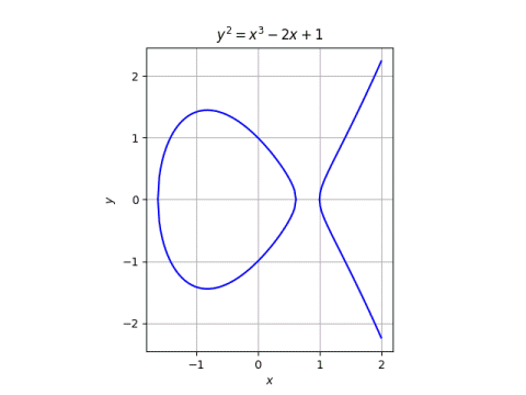
Elliptic curves are very concrete. There are some subtleties in the definition—more on that in a moment—but they’re essentially the set of point satisfying a simple equation. And yet a lot of extremely abstract mathematics has been developed out of necessity to study these simple objects. And while the objects are in some sense simple, the questions that people naturally ask about them are far from simple.

y^2 = x^3 - 2x + 1

Preliminary definition

A preliminary definition of an elliptic curve is the set of points satisfying

y² = x³ + ax + b.

This is a theorem, not a definition, and it requires some qualifications. The values xya, and b come from some field, and that field is an important part of the definition of an elliptic curve. If that field is the real numbers, then all elliptic curves do have the form above, known as the Weierstrass form. For fields of characteristic 2 or 3, the Weierstrass form isn’t general enough. Also, we require that

4a³ + 27b² ≠ 0.

The other day I wrote about Curve1174, a particular elliptic curve used in cryptography. The points on this curve satisfy

x² + y² = 1 – 1174 x² y²

This equation does not specify an elliptic curve if we’re working over real numbers. But Curve1174 is defined over the integers modulo p = 2251 – 9. There it is an elliptic curve. It is equivalent to a curve in Weierstrass, though that’s not true when working over the reals. So whether an equation defines an elliptic curve depends on the field the constituents come from.

Not an ellipse, not a curve

An elliptic curve is not an ellipse, and it may not be a curve in the usual sense.

There is a connection between elliptic curves and ellipses, but it’s indirect. Elliptic curves are related to the integrals you would write down to find the length of a portion of an ellipse.

Working over the real numbers, an elliptic curve is a curve in the geometric sense. Working over a finite field, an elliptic curve is a finite set of points, not a continuum. Working over the complex numbers, an elliptic curve is a two-dimensional surface. The name “curve” is extended by analogy to elliptic curves over general fields.

Final definition

In this section we’ll give the full definition of an algebraic curve, though we’ll be deliberately vague about some of the details.

The definition of an elliptic curve is not in terms of equations of a particular form. It says an elliptic curve is a

  • smooth,
  • projective,
  • algebraic curve,
  • of genus one,
  • having a specified point O.

Working over real numbers, smoothness can be specified in terms of derivatives. But that does smoothness mean working over a finite field? You take the derivative equations from the real case and extend them by analogy to other fields. You can “differentiate” polynomials in settings where you can’t take limits by defining derivatives algebraically. (The condition 4a³ + 27b² ≠ 0 above is to guarantee smoothness.)

Informally, projective means we add “points at infinity” as necessary to make things more consistent. Formally, we’re not actually working with pairs of coordinates (xy) but equivalence classes of triples of coordinates (x, yz). You can usually think in terms of pairs of values, but the extra value is there when you need it to deal with points at infinity. More on that here.

An algebraic curve is the set of points satisfying a polynomial equation.

The genus of an algebraic curve is roughly the number of holes it has. Over the complex numbers, the genus of an algebraic curve really is the number of holes. As with so many ideas in algebra, a theorem from a familiar context is taken as a definition in a more general context.

The specified point O, often the point at infinity, is the location of the identity element for the group addition. In the post on Curve1174, we go into the addition in detail, and the zero point is (0, 1).

In elliptic curve cryptography, it’s necessary to specify another point, a base point, which is the generator for a subgroup. This post gives an example, specifying the base point on secp256k1, a curve used in the implementation of Bitcoin.

Microsoft replacing SHA-1

According to this article, Microsoft is patching Windows 7 and Windows Server 2008 to look for SHA-2 hash functions of updates. These older versions of Windows have been using SHA-1, while newer version are already using SHA-2.

This is a good move, but unnecessary. Here’s what I mean by that. The update was likely unnecessary for reasons I’ll explain below, but it was easy to do, and it increased consistency across Microsoft’s product line. It’s also good PR.

What are SHA-1 and SHA-2?

Let’s back up a bit. SHA-1 and SHA-2 are secure hash functions [1]. They take a file, in this case a Microsoft software update, and return a relatively small number, small relative to the original file size. In the case of SHA-1, the result is 160 bits (20 bytes).  They’re designed so that if a file is changed, the function value is nearly certain to change. That is, it’s extremely unlikely that a change to the file would not result in a change to the hash value.

The concern isn’t accidental changes. The probability of accidentally producing two files with the same hash function value is tiny as I show here.

The concern is a clever attacker who could modify the software update in such a way that the hash function remains unchanged, bypassing the hash as a security measure. That would be harder to do with SHA-2 than with SHA-1, hence Microsoft’s decision years ago to move to SHA-2 for new versions of the operating system, and its recent decision to make the change retroactive.

How hard is it to produce collisions?

By a collision we mean two files that hash to the same value. It’s obvious from the pigeon hole principle [2] that collisions are possible, but how hard are they to produce deliberately?

Google demonstrated two years ago that it could produce two PDF files with the same SHA-1 hash value. But doing so required over 6,500 years of CPU time running in parallel [3]. Also, Google started with a file designed to make collisions possible. According to their announcement,

We started by creating a PDF prefix specifically crafted to allow us to generate two documents with arbitrary distinct visual contents, but that would hash to the same SHA-1 digest.

It would be harder to start with a specified input, such as a software update file and generate a collision. It would be harder still to generate a collision that had some desired behavior.

According to this page, it’s known how to tamper with two files simultaneously so that they will have the same SHA-1 hash values. This is what Google did, at the cost of thousands of CPU years. But so far, nobody has been able to start with a given file and create another file with the same SHA-1 value. (Update: Now they have!)

As I said at the beginning, it made sense for Microsoft to decide to move from SHA-1 to SHA-2 because the cost of doing so was small. But the use of SHA-1 hash codes is probably not the biggest security risk in Windows 7.

More secure hash posts

[1] SHA-1 is a hash function, but SHA-2 is actually a family of hash functions: SHA-224, SHA-256, SHA-384, SHA-512, SHA-512/224, and SHA-512/256. All are believed to provide at least 112 bits of security, while SHA-1 provides less than 63.

The SHA-x functions output x bits. The SHA-x/y functions use x bits of internal state and output y bits. To be consistent with this naming convention, SHA-1 should be called SHA-160.

[2] The pigeon hole principle says that if you put more than n things into n boxes, one of the boxes has to have more than one thing. If you hash files of more than n bits to n-bit numbers, at least two files have to go to the same value.

[3] If you were to rent this much CPU time in the cloud at 5 cents per CPU hour, it would cost about $2,800,000. If the only obstacle were the cost of computing resources, someone might be willing to pay that to tamper with a Microsoft update. (Update: with a new algorithm announced in January 2020, the estimated cost has dropped $45,000.)

Hash function menagerie

Here’s an oversimplified survey of cryptographic hash functions: Everyone used to use MD5, now they use some variation on SHA.

There’s some truth to that. MD5 was very popular, and remains popular years after it was proven insecure. And now variations on SHA like SHA1 and SHA256 are commonly used. But there are a lot more cryptographic hash functions in common use.

Python support

If Python’s hashlib is a reliable guide, the most common hashing algorithms are

  • MD5
  • SHA1
  • SHA224
  • SHA256
  • SHA384
  • SHA512

because these are the six algorithms guaranteed to be supported on every platform, as listed in the output of the algorithms_guaranteed method in hashlib.

The algorithms_available methods in hashlib includes additional algorithms available in a particular installation. On the computer I’m using at the moment, it lists 18 hash algorithms in addition to those on the guaranteed list.

Mathematica support

Mathematica supports the hash functions on hashlib‘s guaranteed list, and a few more:

  • Adler32
  • CRC32
  • MD3
  • MD4
  • RIPEMD160
  • RIPEMD160SHA256
  • SHA256SHA256

The first two hashes, Adler32 and CRC32, were never intended to be secure. They were designed simply as error detection codes and weren’t designed to be tamper-resistant. As the names imply, MD3 and MD4 were predecessors to MD5.

The hash that Mathematica calls RIPEMD160SHA256 is SHA 256 followed by the RIPEMD160. The reason this combination gets a name of its own is because it is used in Bitcoin. Finally, SHA256SHA256 is simply SHA256 applied twice.

The long tail

The hash functions mentioned above are the most commonly used, but there are hundreds of others in common use. The hashcat password cracking tool lists 260 kinds of hash functions it can attack.

Some of these hash functions are fundamental algorithms, such as Whirlpool and variations of GOST. Some are combinations of primitive functions, such as salted or iterated variations. Many of them are vendor and product specific. For example, hashcat lists nine different hashing algorithms associated with various versions of Microsoft Office, six algorithms for Cisco products, five algorithms for SAP, etc.

It’s interesting to speculate on why there are so many custom hash functions: hashing technology progress, differing emphases on security and speed, not-invented-here syndrome, etc.

Security by variety

There’s something going on that isn’t exactly security-by-obscurity, i.e. relying on keeping your encryption algorithm a secret. The hashing algorithms for all the products mentioned above are well known, but there may be some small advantage to being a little bit off the beaten path.

People have built special hardware and software for attacking popular hashing algorithms, and doing something a little different could prevent this from working on your hash. Of course doing something a little different could also introduce a weakness you didn’t anticipate. Creating your own encryption algorithm is a bad idea unless you’re an expert, and often even if you are an expert But making a new hash function by combining secure primitives is not as dangerous as creating your own encryption algorithm.

More hash function posts

Addition on Curve1174

I’ve written about elliptic curve and alluded to the fact that there’s a special kind of addition for points on the curve. But I haven’t gone into details because it’s more complicated than I wanted to get into.

However, there’s a special case where the details are not complicated, the so called Edwards curves. I’ll look briefly at Edwards curves in general, then focus on Curve1174, a particular Edwards curve used in cryptography.

The example here could be used in an introductory group theory course with no reference to elliptic curves. Just think of it as a funny way to add pairs of integers.

Addition on Edwards curves

For a particular class of elliptic curve, Edwards curves, the addition formula is simpler than usual. As mentioned a few days ago, an Edwards curve has the form

x² + y² = 1 + d x² y²

where d is not 0 or 1 in the underlying finite field. Then addition on the curve is given by

(x_1,y_1) + (x_2,y_2) = \left( \frac{x_1 y_2 + x_2 y_1}{1 + dx_1 x_2 y_1 y_2}, \frac{y_1 y_2 - x_1 x_2}{1 - dx_1 x_2 y_1 y_2} \right)

When d is a square, there are some exceptions. When d is not a square, as will be the case in our application, the denominators are never zero, and so the formula above is all there is to the addition rule.

Note that the division in the formula above is division in the underlying finite field, i.e. multiplication by the multiplicative inverse.

Curve1174

We’re interested in Curve1174, a particular elliptic curve used in cryptography. The underlying field is GF(p), the integers modulo the prime p = 2251 – 9. Also, d = -1174, from whence the curve takes its name.

Plotting Curve1174 over the reals

The plot above shows what Curve1174 looks like over the real numbers, though we’re interested in the curve over the integers mod p. (By the way, if d > 0 you get a curve that looks like a squircle.)

We consider the pairs of integers (x, y) that lie on the curve, i.e. those that satisfy

x² + y² = 1 + d x² y² mod p.

You can show that the sum of two points on the curve is another point on the curve, if you define addition with the formula above. The identity element for addition is the pair (0, 1). The additive inverse of a point (xy) is the point (-xy). So we have a group. Addition is commutative, and so in fact we have an Abelian group.

Python code

We can implement addition on Curve1174 in a few lines of Python.

from sympy import mod_inverse

def divide(a, b, p):
    "Compute a/b in GF(p)"
    return (a*mod_inverse(b, p))%p

def group_add(x1, y1, x2, y2, p, d):
    x3 = divide(x1*y2 + x2*y1, 1 + d*x1*x2*y1*y2, p)
    y3 = divide(y1*y2 - x1*x2, 1 - d*x1*x2*y1*y2, p)
    return (x3, y3)

The only thing we needed SymPy for was the mod_inverse function. It wouldn’t take much work to write your own mod_inverse function from scratch using the method outlined here using a variation on the Euclidean algorithm.

It’s clear that (1, 0) is a point on the curve, and so we can add it to itself with the code

p = 2**251 - 9
d = -1174
print(group_add(1, 0, 1, 0, p, d))

and find that it equals

(0, 3618502788666131106986593281521497120414687020801267626233049500247285301238),

which may come as a bit of a surprise. Arithmetic here is not intuitive; it scrambles up points well, which hints at why the curve is useful in cryptography.

Let’s find another point on the curve. Let’s set x = 2019 and see what y is. When we come up with the equation y must satisfy, the Jacobi symbol shows there is no solution.

When x = 2025 there is a solution, and we can compute it using sqrt_mod from sympy.ntheory.

x = 2025
k = divide(1 - x*x, 1 - d*x*x, p)
y = sqrt_mod(k, p)

This says the point

(2025, 588747530266665079407582947937120321357732884331117971504880828350684014295)

is on Curve1174. And since x and y only appear as squares in the equation defining the curve, once we find an (x, y) pair on the curve, the points (±x, ±y) are also on the curve.

Just for grins, let’s double the point (xy) above, i.e. add it to itself. This works out to

(2795920935947049934301363619759082573282734750667150130900931245990107374027,  2577351770662637935098262284237063829290291047539093190165388036658162531660).

Number of points on Curve1174

In general it can be hard to compute how many point lie on an elliptic curve, but in the case of Curve 1174 the number of points is known. Bernstein et al computed that the number of points on Curve1174 is p + 1 – t where t is a big number, but much smaller than p, on the order of the square root of p. Specifically,

t = 45330879683285730139092453152713398836.

Why not just absorb the 1 into t? This was done to match the notation in Hasse’s theorem. See the footnote here.

Elliptic curve cryptography (ECC)

What does all this have to do with cryptography? Cryptographers like to find problems that can be computed easily but that are hard to reverse. Most public key cryptography methods depend on the difficulty of undoing one of three things:

  • multiplication,
  • modular exponentiation, or
  • multiplication over an elliptic curve.

RSA encryption, for example, depends on the difficulty of factoring the product of two large primes.

The elliptic curve discrete logarithm problem (ECDLP) is the problem of undoing multiplication over an elliptic curve. If n is an integer and P is a point on the curve, we can compute QnP easily. If n is large, we don’t just add P to itself n times. Instead we double it log2n times and add the necessary intermediate results, analogous to fast exponentiation.

It’s easy to compute Q given n and P, but it’s hard to compute n given P and Q. This is the elliptic curve discrete logarithm problem that EEC protocols rely on for their security.

More elliptic curve cryptography posts

The hard part in becoming a command line wizard

I’ve long been impressed by shell one-liners. They seem like magical incantations. Pipe a few terse commands together, et voilà! Out pops the solution to a problem that would seem to require pages of code.

Source http://dilbert.com/strip/1995-06-24

Are these one-liners real or mythology? To some extent, they’re both. Below I’ll give a famous real example. Then I’ll argue that even though such examples do occur, they may create unrealistic expectations.

Bentley’s exercise

In 1986, Jon Bentley posted the following exercise:

Given a text file and an integer k, print the k most common words in the file (and the number of their occurrences) in decreasing frequency.

Donald Knuth wrote an elegant program in response. Knuth’s program runs for 17 pages in his book Literate Programming.

McIlroy’s solution is short enough to quote below [1].

    tr -cs A-Za-z '
    ' |
    tr A-Z a-z |
    sort |
    uniq -c |
    sort -rn |
    sed ${1}q

McIlroy’s response to Knuth was like Abraham Lincoln’s response to Edward Everett at Gettysburg. Lincoln’s famous address was 50x shorter than that of the orator who preceded him [2]. (Update: There’s more to the story. See [3].)

Knuth and McIlroy had very different objectives and placed different constraints on themselves, and so their solutions are not directly comparable. But McIlroy’s solution has become famous. Knuth’s solution is remembered, if at all, as the verbose program that McIlroy responded to.

The stereotype of a Unix wizard is someone who could improvise programs like the one above. Maybe McIlroy carefully thought about his program for days, looking for the most elegant solution. That would seem plausible, but in fact he says the script was “written on the spot and worked on the first try.” He said that the script was similar to one he had written a year before, but it still counts as an improvisation.

Why can’t I write scripts like that?

McIlroy’s script was a real example of the kind of wizardry attributed to Unix adepts. Why can’t more people quickly improvise scripts like that?

The exercise that Bentley posed was the kind of problem that programmers like McIlroy solved routinely at the time. The tools he piped together were developed precisely for such problems. McIlroy didn’t see his solution as extraordinary but said “Old UNIX hands know instinctively how to solve this one in a jiffy.”

The traditional Unix toolbox is full of utilities for text manipulation. Not only are they useful, but they compose well. This composability depends not only on the tools themselves, but also the shell environment they were designed to operate in. (The latter is why some utilities don’t work as well when ported to other operating systems, even if the functionality is duplicated.)

Bentley’s exercise was clearly text-based: given a text file, produce a text file. What about problems that are not text manipulation? The trick to being productive from a command line is to turn problems into text manipulation problems.  The output of a shell command is text. Programs are text. Once you get into the necessary mindset, everything is text. This may not be the most efficient approach to a given problem, but it’s a possible strategy.

The hard part

The hard part on the path to becoming a command line wizard, or any kind of wizard, is thinking about how to apply existing tools to your particular problems. You could memorize McIlroy’s script and be prepared next time you need to report word frequencies, but applying the spirit of his script to your particular problems takes work. Reading one-liners that other people have developed for their work may be inspiring, or intimidating, but they’re no substitute for thinking hard about your particular work.

Repetition

You get faster at anything with repetition. Maybe you don’t solve any particular kind of problem often enough to be fluent at solving it. If someone can solve a problem by quickly typing a one-liner in a shell, maybe they are clever, or maybe their job is repetitive. Or maybe both: maybe they’ve found a way to make semi-repetitive tasks repetitive enough to automate. One way to become more productive is to split semi-repetitive tasks into more creative and more repetitive parts.

More command line posts

[1] The odd-looking line break is a quoted newline.

[2] Everett’s speech contained 13,607 words while Lincoln’s Gettysburg Address contained 272, a ratio of almost exactly 50 to 1.

[3] See Hillel Wayne’s post Donald Knuth was Framed. Here’s an excerpt:

Most of the “eight pages” aren’t because Knuth is doing LP [literate programming], but because he’s Donald Knuth:

  • One page is him setting up the problem (“what do we mean by ‘word’? What if multiple words share the same frequency?”) and one page is just the index.
  • Another page is just about working around specific Pascal issues no modern language has, like “how do we read in an integer” and “how do we identify letters when Pascal’s character set is poorly defined.”
  • Then there’s almost four pages of handrolling a hash trie.

The “eight pages” refers to the length of the original publication. I described the paper as 17 pages because that the length in the book where I found it.

Naming elliptic curves used in cryptography

There are an infinite number of elliptic curves, but a small number that are used in elliptic curve cryptography (ECC), and these special curves have names. Apparently there are no hard and fast rules for how the names are chosen, but there are patterns.

The named elliptic curves are over a prime field, i.e. a finite field with a prime number of elements p, denoted GF(p). The number of points on the elliptic curve is on the order of p [1].

The curve names usually contain a number which is the number of bits in the binary representation of p. Let’s see how that plays out with a few named elliptic curves.

Curve name Bits in p
ANSSI FRP256v1   256
BN(2, 254) 254
brainpoolP256t1   256
251
255
Curve383187 383
E-222 222
E-382 382
E-521 521
448
M-211 221
M-383 383
M-511 511
NIST P-224 224
256
384
256

In Curve25519, p = 2255 – 19 and in Curve 383187, p = 2383 – 187. Here the number of bits in p is part of the name but another number is stuck on.

The only mystery on the list is Curve1174 where p has 251 bits. The equation for the curve is

x² + y² = 1 – 1174 y²

and so the 1174 in the name comes from a coefficient rather than from the number of bits in p.

Edwards curves

The equation for Curve1174 doesn’t look like an elliptic curve. It doesn’t have the familiar (Weierstrass) form

y² = x³ + ax + b

It is an example of an Edwards curve, named after Harold Edwards. So are all the curves above whose names start with “E”. These curves have the form

x² + y² = 1 + d x² y².

where d is not 0 or 1. So some Edwards curves are named after their d parameter and some are named after the number of bits in p.

It’s not obvious that an Edwards curve can be changed into Weierstrass form, but apparently it’s possible; this paper goes into the details.

The advantage of Edwards curves is that the elliptic curve group addition has a simple, convenient form. Also, when d is not a square in the underlying field, there are no exceptional points to consider for group addition.

Is d = -1174 a square in the field underlying Curve1174? For that curve p = 2251 – 9, and we can use the Jacobi symbol code from earlier this week to show that d is not a square.

    p = 2**251 - 9
    d = p-1174
    print(jacobi(d, p))

This prints -1, indicating that d is not a square. Note that we set d to p – 1174 rather than -1174 because our code assumes the first argument is positive, and -1174 and p – 1174 are equivalent mod p.

Update: More on addition on Curve1174.

Prefix conventions

A US government publication (FIPS PUB 186-4) mandates the following prefixes:

  • P for curves over a prime field,
  • B for curves over a binary field (i.e. GF(2n)), and
  • K for Koblitz fields.

The ‘k’ in secp256k1 also stands for Koblitz.

The M prefix above stands for Montgomery.

More ECC posts

[1] It is difficult to compute the exact number of points on an elliptic curve over a prime field. However, the number is roughly p ± 2√p. More precisely, Hasse’s theorem says

|\#(E/\mathbb{F}_p) - p - 1| \leq 2\sqrt{p}

Entropy extractor used in μRNG

Yesterday I mentioned μRNG, a true random number generator (TRNG) that takes physical sources of randomness as input. These sources are independent but non-uniform. This post will present the entropy extractor μRNG uses to take non-uniform bits as input and produce uniform bits as output.

We will present Python code for playing with the entropy extractor. (μRNG is extremely efficient, but the Python code here is not; it’s just for illustration.) The code will show how to use the pyfinite library to do arithmetic over a finite field.

Entropy extractor

The μRNG generator starts with three bit streams—X, Y, and Z—each with at least 1/3 bit min-entropy per bit.

Min-entropy is Rényi entropy with α = ∞. For a Bernoulli random variable, that takes on two values, one with probability p and the other with probability 1-p, the min-entropy is

-log2 max(p, 1-p).

So requiring min-entropy of at least 1/3 means the two probabilities are less than 2-1/3 = 0.7937.

Take eight bits (one byte) at a time from XY, and Z, and interpret each byte as an element of the finite field with 28 elements. Then compute

X*YZ

in this field. The resulting stream of bits will be independent and uniformly distributed, or very nearly so.

Purified noise

Just a quick aside. Normally you want to remove noise from data to reveal a signal. Said another way, you want to split the data into signal and noise so you can throw out the noise. Here the goal is the opposite: we want to remove any unwanted signal in order to create pure noise!

Python implementation

We will need the bernoulli class for generating our input bit streams, and the pyfinite for doing finite field arithmetic on the bits.

    from scipy.stats import bernoulli
    from pyfinite import ffield

And we will need a couple bit manipulation functions.

    def bits_to_num(a):
        "Convert an array of bits to an integer."
    
        x = 0
        for i in range(len(a)):
            x += a[i]*2**i
        return x

    def bitCount(n):
        "Count how many bits are set to 1."
        count = 0
        while(n):
            n &= n - 1
            count += 1
        return count 

The following function generates random bytes using the entropy extractor. The input bit streams have p = 0.79, corresponding to min-entropy 0.34.

    def generate_byte():
        "Generate bytes using the entropy extractor."
    
        b = bernoulli(0.79)
    
        x = bits_to_num(b.rvs(8))
        y = bits_to_num(b.rvs(8))
        z = bits_to_num(b.rvs(8)) 

        F = ffield.FField(8)
        return F.Add(F.Multiply(x, y), z)

Note that 79% of the bits produced by the Bernoulli generator will be 1’s. But we can see that the output bytes are about half 1’s and half 0’s.

    s = 0
    N = 1000
    for _ in range(N):
        s += bitCount( generate_byte() )
    print( s/(8*N) )

This returned 0.50375 the first time I ran it and 0.49925 the second time.

For more details see the μRNG paper.

Update: RNG test suite results

I ran an experiment, creating streams of biased data and running them through the entropy extractor. The first post in the series, NIST STS, explains the set up. The last post in the series, using TestU01, summarizes the results. In a nutshell, the extractor passes STS and DIEHARDER, but fails PractRand and TestU01.

Related posts

Solving for probability given entropy

If a coin comes up heads with probability p and tails with probability 1-p, the entropy in the coin flip is

S = –p log2 p – (1-p) log2 (1-p).

It’s common to start with p and compute entropy, but recently I had to go the other way around: given entropy, solve for p. It’s easy to come up with an approximate solution.

entropy and approximation

Entropy in this case is approximately quadratic

S ≈ 4p(1-p)

and so

p ≈ (1 ± √(1-S))/2.

This is a good approximation if S is near 0 or 1 but mediocre in the middle. You could use solve for p numerically, say with Newton’s method, to get more accuracy if needed.

Update

As Sjoerd Visscher pointed out in the comments, the quadratic approximation for entropy is much better if you raise it to the power 3/4. When I added this new approximation to the graph above, the new approximation agreed with the correct value to within the thickness of the plotting line.

To make the approximation error visible, here’s the log of the absolute value of the error of the two approximations, on a log scale.

approximation error on log scale

The error in the new approximation is about an order of magnitude smaller, sometimes more.

The improved approximation for entropy is

S ≈ (4p(1-p))3/4

and so the new approximation for probability is

p ≈ (1 ± √(1-S4/3))/2.

More information theory posts