Recovering the state of xorshift128

I’ve written a couple posts lately about reverse engineering the internal state of a random number generator, first Mersenne Twister then lehmer64. This post will look at xorshift128, implemented below.

import random

# Seed the generator state
a: int = random.getrandbits(32)
b: int = random.getrandbits(32)
c: int = random.getrandbits(32)
d: int = random.getrandbits(32)

MASK = 0xFFFFFFFF

def xorshift128() -> int:
    global a, b, c, d

    t = d
    s = a

    t ^= (t << 11) & MASK t ^= (t >>  8) & MASK
    s ^= (s >> 19) & MASK

    a, b, c, d = (t ^ s) & MASK, a, b, c

    return a

Recovering state

Recovering the internal state of the generator is simple: it’s the four latest outputs in reverse order. This is illustrated by the following chart.

 a b c d output 5081e5ca 79259a41 63e12955 651e537d c793d11c c793d11c 5081e5ca 79259a41 63e12955 ad52e33a ad52e33a c793d11c 5081e5ca 79259a41 f8f09343 f8f09343 ad52e33a c793d11c 5081e5ca a7009622 a7009622 f8f09343 ad52e33a c793d11c fe42a8ef

This means that once we’ve seen four outputs, we can predict the rest of the outputs. The following code demonstrates this.

Let’s generate five random values.

out = [xorshift128() for _ in range(5)]

Running

print(hex(out[4]))

shows the output 0xc3f4795d.

If we reset the state of the generator using the first four outputs

d, c, b, a, _ = out
print(hex(xorshift128()))

we get the same result.

Good stats, bad security

Mersenne Twister and lehmer64 have good statistical properties, despite being predictable. The xorshift128 generator is even easier to predict, but it also has good statistical properties. These generators would be fine for many applications, such as Monte Carlo simulation, but disastrous for use in cryptography.

The post on lehmer64 mentioned at the end that the internal state of PCG64 can also be recovered from its output. However, doing so requires far more sophisticated math and thousands of hours of compute time. Still, it’s not adequate for cryptography. For that you’d need a random number generator designed to be secure, such as ChaCha.

So why not just use a cryptographically secure random number generator (CSPRNG) for everything? You could, but the other generators mentioned in this post use less memory and are much faster. PCG64 occupies an interesting middle ground: simple and fast, but not easily reversible.

Hacking the lehmer64 RNG

A couple days ago I wrote about hacking the Mersenne Twister. I explained how to recover the random number generator’s internal state from a stream of 640 outputs.

This post will do something similar with the lehmer64 random number generator. This generator is very simple to implement. Daniel Lemire found it to be “the fastest conventional random number generator that can pass Big Crush,” a well-respected test for pseudorandom number generators.

Implementing lehmer64

The lehmer64 generator can be implemented in C by

__uint128_t g_lehmer64_state;

uint64_t lehmer64() {
    g_lehmer64_state *= 0xda942042e4dd58b5ULL;  
  return g_lehmer64_state >> 64;
}

The analogous code in Python would have to simulate the overflow behavior of a 128-bit integer by reducing the state mod 2128 after the multiplication.

Reverse engineering lehmer64 is easier than reverse engineering the Mersenne Twister because only three outputs are needed. However, the theory behind the exploit is more sophisticated. See [1].

The following code sets the state to an arbitrary initial seed value and generates three values.

#include <stdio.h>
#include <stdint.h>

int main(void)
{
    g_lehmer64_state = 0x4789499d78770934; // seed
    for (int i = 0; i < 3; i++) {
        printf("0x%016lx\n", lehmer64());
    }

    return 0;
}

The code prints the following.

0x3d144d12822bcc2e
0x85a67226191a568d
0x53e803dffc88e8f8

Exploiting lehmer64

Here is Python code for recovering the state of the lehmer64 generator given in [1].

def reconstruct(X):
    a = 0xda942042e4dd58b5
    r = round(2.64929081169728e-7 * X[0] + 3.51729342107376e-7 * X[1] + 3.89110109147656e-8 * X[2])
    s = round(3.12752538137199e-7 * X[0] - 1.00664345453760e-7 * X[1] - 2.16685184476959e-7 * X[2])
    t = round(3.54263598631140e-8 * X[0] - 2.05535734808162e-7 * X[1] + 2.73269247090513e-7 * X[2])
    u = r * 1556524 + s * 2249380 + t * 1561981
    v = r * 8429177212358078682 + s * 4111469003616164778 + t * 3562247178301810180
    state = (a*u + v) % (2**128)
    return state

Let’s call reconstruct with the output of our C code.

X = [0x3d144d12822bcc2e, 0x85a67226191a568d, 0x53e803dffc88e8f8]
print( hex( reconstruct(X) ) )

This prints

0x3d144d12822bcc2e1b81101c593761c4

Now for the confusing part: at what point is the number above the state of the generator? Is it the state before or after generating the three values? Neither! It is the state after generating the first value.

We can verify this by modifying the C code as follows and rerunning it.

void print_u128(__uint128_t n)
{
    printf("0x%016lx%016lx\n",
           (uint64_t)(n >> 64),      // upper 64 bits
           (uint64_t)n);             // lower 64 bits
}

int main(void)
{
    g_lehmer64_state = 0x4789499d78770934; // seed
    for (int i = 0; i < 3; i++) {
        printf("0x%016lx\n", lehmer64());
        printf("state: ");
        print_u128(g_lehmer64_state);
    }
 
    return 0;
}

The main goal of [1] is to recover the state of the PCG generator, not the lehmer64 generator. The latter was a side quest. Recovering the state of PCG64 is much harder; the authors estimate it takes about 20,000 CPU-hours. The paper shows that a technique used as part of pursuing their main goal can quickly recover the lehmer64 state.

Related posts

[1] Charles Bouillaguet, Florette Martinez, and Julia Sauvage. Practical seed-recovery for the PCG Pseudo-Random Number Generator. IACR Transactions on Symmetric Cryptology. ISSN 2519-173X, Vol. 2020, No. 3, pp. 175–196.

Reverse engineering Mersenne Twister with Linear Algebra

The Mersenne Twister (MT) is a random number generator with good statistical properties but bad cryptographic properties. In buzzwords, it’s a PRNG but not a CSPRNG.

This post will show how the internal state of a MT generator can be recovered from its output. We’ll do this using linear algebra. The bit twiddling approach is more common and more efficient, but the linear algebra approach is conceptually simpler.

How MT works

There are numerous variations on the Mersenne Twister. We’ll focus on the original version that had internal state consists of vector x of length 640 filled with 32-bit numbers. The ideas in this post would apply equally to all MT versions.

The first call to MT returns a “tempered” version of x[0]. The next call returned a tempered version of x[1], and so on. After every 640 calls, the state is scrambled. This scrambling is where the “twist” in the name Mersenne Twister comes from. (The Mersenne part comes from the fact that the period of an MT generator is a Mersenne prime.)

Tempering

Here is Python code for performing the tempering step.

def temper(y):
    y ^= (y >> 11) 
    y ^= (y <<  7) & 0x9d2c5680 
    y ^= (y << 15) & 0xefc60000 
    y ^= (y >> 18)  
    return y

Each step is reversible, and so the temper function is reversible.

Because the tempering step is reversible, the first output can be used to infer the first element of the internal state, the second output to infer the second element, and so on. After 640 calls one can know the entire internal state and predict the rest of the generator’s output from then on.

Linear algebra

The bitwise operations above all correspond to linear operations over GF(2), the field with just two elements, 0 and 1. Addition in this field is XOR and multiplication is AND.

Each step corresponds to multiplying a vector of 32 bits on the left by a 32 × 32 matrix with entries that are 0’s and 1’s, with the understanding that the sum of two bits is their XOR and the product of two bits is their AND. Equivalently, arithmetic is carried out mod 2. So you can compute the matrix-vector product as ordinary integers if you then reduce every integer mod 2.

We will find the matrix M that corresponds to the temper operation and prove that it is invertible by finding its inverse. This proves that tempering is invertible, and one could compute the inverse of tempering by multiplying by M−1, though it would be more efficient to undo tempering by bit twiddling.

One way to recover a matrix is to multiplying by unit vectors ei where the ith component of ei is 1 and the rest of the components are zero. Then

M ei

is the ith column of M.

So we can find the nth column of M by tempering 1 << n = 2n.

M = np.zeros((32, 32), dtype=int)
for i in range(32):
    t = temper(1 << (31-i))
    s = f"{t:032b}"
    for j in range(32):
        M[j, i] = int(s[j])

Let’s generate a random number and compute its tempered form two ways: directly and matrix multiplication.

x = random.getrandbits(32)
y = temper(x)
print(f"{y:032b}")

vx = np.array([int(b) for b in f"{x:032b}"]) # vector form of x
vy = M @ vx % 2 # vector form of y
print("".join(str(b) for b in vy))

Both produce the same bits:

10100101100101101100110101000110
10100101100101101100110101000110

We can find the matrix representation of the untemper function by inverting the matrix M. However, we need to invert it over the field GF(2), not over the integers or reals.

import galois
GF2 = galois.GF(2)
Minv = np.linalg.inv(GF2(M))

Here are visualizations of M and its inverse using a black square for a 1 and a white square for a 0.

M:

M−1:

The next post will back up and look at the linear algebra of the components that comprise the Mersenne Twister.

Random spherical coordinates

The topic of generating random points on a unit sphere has come up several times here. The standard method using normal random samples generates points (x, y, z) in Cartesian coordinates.

If you wanted points in spherical coordinates, you could first generate points in Cartesian coordinates, then convert the points to spherical coordinates. But it would seem more natural, and possibly more efficient, to directly generate spherical coordinates (ρ, θ, ϕ). That’s what we’ll do in this post.

Unfortunately there are several conventions for spherical coordinates, as described here, so we should start by saying we’re using the math convention that (ρ, θ, ϕ) means (radius, longitude, polar angle). The polar angle ϕ is 0 at the north pole and π at the south pole.

Generating the first two spherical coordinate components is trivial. On a unit sphere, ρ = 1, and θ we generate uniformly on [0, 2φ]. The polar angle ϕ requires more thought. If we simply generated φ uniformly from [0, π] we’d put too many points near the poles and too few points near the equator.

As I wrote about a few days ago, the x, y, and z coordinates of points on a sphere are uniformly distributed. In particular, the z coordinate is uniformly distributed, and so we need cos ϕ to be uniformly distributed, not ϕ itself. We can accomplish this by generating uniform points from [−1, 1] and taking the inverse cosine.

Here’s Python code summarizing the algorithm for generating random points on a sphere in spherical coordinates.

from numpy import random, pi, arccos

def random_pt() # in spherical coordinates
    rho = 1
    theta = 2*pi*random.random()
    phi = arccos(1 - 2*random.random())
    return (rho, theta, phi)

See the next post for a demonstration.

Random samples from a tetrahedron

Exactly one month ago I wrote about sampling points from a triangle. This post will look at the three dimensional analog, sampling from a tetrahedron. The generalization to higher dimensions works as well.

Sampling from a triangle

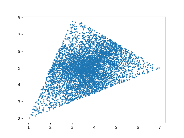
In the triangle post, I showed that a naive approach doesn’t work but a variation does. If the vertices of the triangle are AB, and C, then the naive approach is to generate three uniform random numbers, normalize them, and use them to form a linear combination of the vertices. That is, generate

r1r2r3

uniformly from [0, 1], then define

r1′ = r1/(r1r2r3)
r2′ = r2/(r1r2r3)
r3′ = r3/(r1r2r3)

and return as a random sample the point

r1′ A + r2′ B + r3C.

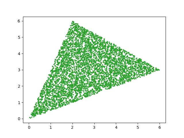
This oversamples points near the middle of the triangle and undersamples points near the vertices. But everything above works if you replace uniform samples with exponential samples.

Sampling from a tetrahedron

The analogous method works for a tetrahedron with vertices ABC, and D. Generate exponential random variables ri for i = 1, 2, 3, 4. Then normalize, defining each ri′ to be ri divided by the sum of all the ri s. Then the random sample is

r1′ A + r2′ B + r3C + r4D.

In the case of the triangle, it was easy to visualize that uniformly generated rs did not lead to uniform samples of the triangle, but that exponentially generated rs did. This is harder to do in three dimensions. Even if the points were uniformly sampled from a tetrahedron, they might not look uniformly distributed from a given perspective.

So how might we demonstrate that our method works? One approach would be to take a cube inside a tetrahedron and show that the proportion of samples that land inside the cube is what we’d expect, namely the ratio of the volume of the cube to the volume of the tetrahedron.

This brings up a couple interesting subproblems.

  1. How do we compute the volume of a tetrahedron?
  2. How can we test whether our cube lies entirely within the tetrahedron?

Volume of a tetrahedron

To find the volume of a tetrahedron, form a matrix M whose columns are the vectors from three of the vertices to the remaining vertex. So we could take AD, BD, and CD. The volume of the tetrahedron is the determinant of M divided by 6.

Testing whether a cube is inside a tetrahedron

A tetrahedron is convex, and so the line segment joining any two points inside the tetrahedron lies entirely inside the tetrahedron. It follows that if all the vertices of a cube are inside the a tetrahedron, the entire cube is inside.

So this brings us to the problem of testing whether a point is inside a tetrahedron. We can do this by converting the coordinates of the point to barycentric coordinates, then testing whether all the coordinates are non-negative and add to 1.

Random sampling illustration

I made up four points as vertices of a tetrahedron.

import numpy as np

A = [0, 0, 0]
B = [5, 0, 0]
C = [0, 7, 0]
D = [0, 1, 6]
A, B, C, D = map(np.array, [A, B, C, D])

For my test cube I chose the cube whose vertex coordinates are all combinations of 1 and 2. So the vertex nearest the origin is (1, 1, 1) and the vertex furthest from the origin is (2, 2, 2). You can verify that all the vertices are inside the tetrahedron, and so the cube is inside the tetrahedron.

The tetrahedron has volume 35, and the cube has volume 1, so we expect 1/35th of the random points to land inside the cube. Here’s the code to sample the tetrahedron and calculate the proportion of points that land in the cube.

from scipy.stats import expon

def incube(v):
    return 1 <= v[0] <= 2 and 1 <= v[1] <= 2 and 1 <= v[2] <= 2

def good_sample(A, B, C, D):
    r = expon.rvs(size=4)
    r /= sum(r)
    return r[0]*A + r[1]*B + r[2]*C + r[3]*D

def bad_sample(A, B, C, D):
    r = np.random.random(size=4)
    r /= sum(r)
    return r[0]*A + r[1]*B + r[2]*C + r[3]*D

N = 1_000_000

badcount  = 0
goodcount = 0

for _ in range(N):
    v = bad_sample(A, B, C, D)
    if incube(v):
        badcount += 1        
    v = good_sample(A, B, C, D)
    if incube(v):
        goodcount += 1

print(badcount/N, goodcount/N, 1/35)

This produced

0.094388 0.028372 0.028571…

The good (exponential) method match the expected proportion to three decimal places but the bad (uniform) method put about 3.3 times as many points in the cube as expected.

Note that three decimal agreement is about what we’d expect via the central limit theorem since 1/√N = 0.001.

If you’re porting the sampler above to an environment where you don’t a function for generating exponential random samples, you can roll your own by returning −log(u) where u is a uniform sample from [0. 1].

More general 3D regions

After writing the post about sampling from triangles, I wrote a followup post about sampling from polygons. In a nutshell, divide your polygon into triangles, then randomly select a triangle in proportion to its area, then sample with that triangle. You can do the analogous process in three dimensions by dividing a general volume into tetrahedra.

Cycles in Marsaglia’s mental RNG

Last week I wrote about a mental random number generator designed by George Marsaglia. It’s terrible compared to any software RNG, but it produces better output than most people would if asked to say a list of random digits.

Marsaglia’s RNG starts with a two-digit number as a seed state, then at each step replaces n with the 10s digit of n plus 6 times the 1s digit. Here’s the generator in Python form, taken from the earlier post.

state = 42 # Set the seed to any two digit number

def random_digit():
    tens = lambda n: n // 10
    ones = lambda n: n % 10
    global state
    state = tens(state) + 6*ones(state)
    return ones(state)

Only the last digit of the state is returned: the state has two digits but the output has one digit.

Alexander Janßen left an interesting comment on Mastodon regarding the generator:

I’m not sure if it’s already documented anywhere, but a random seed of 59 sticks and always returns a 9. This is similiar to the initial state of 0 (which is more trivial). In return that means, that the state 59 is never reached from any other sequence.

To explore this further, let’s look at just the states of the mental RNG, not the output digits.

If you start with the state 1, you will produce each of the numbers from 1 to 58 in a cycle. It follows that if you start at any number between 1 and 58 you’ll produce the same sequence of states in a cycle, though starting at a different point in the cycle.

… → 1 → 6 → 36 → 39 → … → 1 → …

If you start at 59, you’ll stay at 59 because 5 + 6×9 = 59. In this case, the RNG literally does what is described in the Dilbert cartoon below.

Over here we have our random number generator. nine nine nine nine nine nine ...

Collatz interlude

If you start with a seed larger than 59, you’ll eventually land on a state less than 59, and then produce the same cycle as described above. This is reminiscent of the Collatz conjecture, which I describe here as follows.

The Collatz conjecture asks whether the following procedure always terminates at 1. Take any positive integer n. If it’s odd, multiply it by 3 and add 1. Otherwise, divide it by 2. For obvious reasons the Collatz conjecture is also known as the 3n + 1 conjecture.

The Collatz conjecture remains an open question, though there has been some progress on the problem. I routinely get email from people who say they have no training in math but believe they have solved the problem. Recently they have begun to explain how an LLM led them to their proof.

Does the Collatz sequence get stuck in a cycle for some starting point? Nobody knows. But we can show every starting point for Marsaglia’s mental RNG ends up in a cycle.

Back to Marsaglia

If we start the mental RNG with 99, we next get 63, and then 24. So starting at 99, we end up in a cycle after two steps. The same is true starting at 69 or 89. Otherwise, any starting point between 60 and 98 leads us to a cycle after one step.

Marsaglia’s generator is supposed to be seeded with a two-digit number. What if we seed it with a larger number? For example, what if we start at 1066 and consider the 1os “digit” to be 106?

Each step of the algorithm reduces the state by an order of magnitude, and so if we start with a state greater than 1000, we eventually get to a state less than 1000. Then every state between 100 and 1000 leads to a cycle, usually the permutation of the digits 1 through 58, but the following three-digit states lead to the fixed point of 59.

118, 177, 236, 295, 354, 413, 472, 531, 590

Related posts

Random samples from a polygon

Ted Dunning left a comment on my post on random sampling from a triangle saying you could extend this to sampling from a polygon by dividing the polygon into triangles, and selecting a triangle each time with probability proportional to the triangle’s area.

To illustrate this, let’s start with a irregular pentagon.

To pick a point inside, I used the centroid, the average of the vertices. Connecting the centroid to each of the vertices splits the pentagon into triangles. (Here I implicitly used the fact that this pentagon is convex. The centroid of a non-convex polygon could be outside the polygon.)

We can find the area of the triangles using Heron’s rule.

Here’s what we get for random samples.

Randomly selecting points inside a triangle

If you have a triangle with vertices AB, and C, how would you generate random points inside the triangle ABC?

Barycentric coordinates

One idea would be to use barycentric coordinates.

  1. Generate random numbers α, β, and γ from the interval [0, 1].
  2. Normalize the points to have sum 1 by dividing each by their sum.
  3. Return αA + βB + γC.

This generates points inside the triangle, but not uniformly.

Accept-reject

Another idea is to use an accept-reject method. Draw a rectangle around the triangle, generate points in the square, and throw them away if they land outside the triangle.

An advantage to this method is that it obviously works because it doesn’t rely on anything subtle. Three cheers for brute force!

The method is fairly efficient; on average only half the points will be rejected.

A disadvantage to all accept-reject methods is that they have variable runtime, though this only matters in some applications.

Accept-flip

There is a clever variation on the accept-reject method. Create a parallelogram by attaching a flipped copy of the triangle. Now randomly sample from the parallelogram. Every sample point will either land inside the original triangle or in its flipped twin. If it landed in the original triangle, keep it. If it landed in the twin, flip it back over and use that point.

This is like an accept-reject method, except there’s no waste. Every point is kept, possibly after flipping.

You can find code for implementing this method on Stack Overflow.

Barycentric coordinates fixed

Felix left a note in the comments that the barycentric approach would work if you draw the random weights from an exponential distribution rather than a uniform distribution. That goes against my intuition. I thought about using a different distribution on the weights, but I didn’t work out what it would need to be, but I did not expect it to be exponential. Apparently it works. Here’s a proof by plot:

Related posts

A mental random number generator

Man thinking of random numbers

George Marsaglia was a big name in random number generation. I’ve referred to his work multiple times here, most recently in this article from March on randomly generating points on a sphere. He is best remembered for his DIEHARD battery of tests for RNG quality. See, for example, this post.

I recently learned about a mental RNG that Marsaglia developed. It’s not great, but it’s pretty good for something that’s easy to mentally compute. The output is probably better than if you simply tried to make up random numbers; people are notoriously bad at doing that. Hillel Wayne explores Marsaglia’s method in detail here.

Here’s a summary the generator in Python.

state = 42 # Set the seed to any two digit number

def random_digit():
    tens = lambda n: n // 10
    ones = lambda n: n % 10
    global state
    state = tens(state) + 6*ones(state)
    return ones(state)

Related posts

Legendre and Ethereum

What does an eighteenth century French mathematician have to do with the Ethereum cryptocurrency?

A pseudorandom number generator based on Legendre symbols, known as Legendre PRF, has been proposed as part of a zero knowledge proof mechanism to demonstrate proof of custody in Ethereum 2.0. I’ll explain what each of these terms mean and include some Python code.

The equation x² = a mod p is solvable for some values of a and not for others. The Legendre symbol

\left(\frac{a}{p}\right)

is defined to be 1 if a has a square root mod p, and −1 if it does not. Here a is a positive integer and p is a (large) prime [1]. Note that this is not a fraction, though it looks like one.

As a varies, the Legendre symbols vary randomly. Not literally randomly, of course, but the act random enough to be useful as a pseudorandom number generator.

Legendre PRF

Generating bits by computing Legendre symbols is a lot more work than generating bits using a typical PRNG, so what makes the Legendre PRF of interest to Ethereum?

Legendre symbols can be computed fairly efficiently. You wouldn’t want to use the Legendre PRF to generate billions of random numbers for some numerical integration computation, but for a zero knowledge proof you only need to generate a few dozen bits.

To prove that you know a key k, you can generate a string of pseudorandom bits that depend on the key. If you can do this for a few dozen bits, it’s far more likely that you know the key than that you have guessed the bits correctly. Given k, the Legendre PRF computes

L_k(x) = \frac{1}{2}\left( 1 - \left( \frac{k+x}{p}\right) \right)

for n consecutive values of x [2].

One reason this function is of interest is that it naturally lends itself to multiparty computation (MPC). The various parties could divide up the range of x values that each will compute.

The Legendre PRF has not been accepted to be part of Ethereum 2.o. It’s only been proposed, and there is active research into whether it is secure enough.

Python code

Here’s a little Python scrypt to demonstrate using Lk(x).

    from sympy import legendre_symbol

    def L(x, k, p):
        return (1 - legendre_symbol(x + k, p)) // 2

    k = 20250626
    p = 2**521 - 1
    print([L(x, k, p) for x in range(10)])

This produces the following.

    [1, 1, 1, 1, 0, 0, 1, 0, 0, 1]

Related posts

[1] There is a third possibility: the Legendre symbol equals 0 if a is a multiple of p. We can safely ignore this possibility for this post.

[2] The Legendre symbol takes on the values ±1 and so we subtract this from 1 to get values {0, 2}, then divide by 2 to get bits {0, 1}.