Area of spherical triangle

A few days ago I wrote about how you could calculate the area of a spherical triangle by measuring the angles at its vertices. As was pointed out in the comments, there’s a much more direct way to find the area.

Folke Eriksson gives the following formula for area in [1]. If a, b, and c are three unit vectors, the spherical triangle formed by their vertices has area E where

\tan\left(\frac{E}{2}\right) = \frac{|\mathbf{a} \cdot (\mathbf{b} \times \mathbf{c})|}{1 + \mathbf{a}\cdot \mathbf{b} + \mathbf{b}\cdot \mathbf{c} + \mathbf{a}\cdot \mathbf{c}}

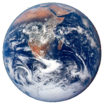
Let’s try the formula out with an example and compare the area to that of a flat triangle. We’ll pick three cities as our three points, assuming the earth is a unit sphere.

Let a = Austin, Texas, b = Boston, Massachusetts, and c = Calgary, Alberta. The spherical coordinates of each point will be (1, θ, φ) where θ is longitude and φ is π/2 minus latitude.

    from numpy import *
    
    def latlong_to_cartesian(latlong):
        phi   = deg2rad( 90 - latlong[0] )
        theta = deg2rad( latlong[1] )
    
        x = sin(phi) * cos(theta)
        y = sin(phi) * sin(thea)
        z = cos(phi)
        return array([x,y,z])
    
    def spherical_area(a, b, c):
        t = abs( inner(a, cross(b, c) ) )
        t /= 1 + inner(a,b) + inner(b,c) + inner(a,c)
        return 2*arctan(t)
    
    def flat_area(a, b, c):
        x = cross(a - b, c - b)
        return 0.5*linalg.norm(x)
    
    # Latitude and longitude
    austin  = (30.2672,  97.7431)
    boston  = (42.3584,  71.0598)
    calgary = (51.0501, 114.0853)
    
    a = latlong_to_cartesian(austin)
    b = latlong_to_cartesian(boston)
    c = latlong_to_cartesian(calgary)
    
    round = spherical_area(a, b, c)
    flat  = flat_area(a, b, c)
    print(round, flat, round/flat)

This shows that our spherical triangle has area 0.0900 and the corresponding Euclidean triangle slicing through the earth would have area 0.0862, the former being 4.467% bigger.

Let’s repeat our exercise with a smaller triangle. We’ll replace Boston and Calgary with Texas cities Boerne and Carrollton.

    boerne  = (29.7947, 98.7320)
    carrollton = (32.9746, 96.8899)

Now we get area 0.000302 in both cases. The triangle is so small relative to the size of the earth that the effect of the earth’s curvature is negligible.

In fact the ratio of the two computed areas is 0.9999, i.e. the spherical triangle has slightly less area. The triangle is so flat that numerical error has a bigger effect than the curvature of the earth.

How could we change our code to get more accurate results for small triangles? That would be an interesting problem. Maybe I’ll look into that in another post.

[1] “On the measure of solid angles”, F. Eriksson, Math. Mag. 63 (1990) 184–187.

Triangles on a pseudosphere

The previous post was about triangles on a sphere. This post will be about triangles on a pseudosphere.

A pseudosphere looks something like the bell of a trumpet or a trombone.

Here’s a plot of a pseudosphere.

This was created in Mathematica with the code

    ParametricPlot3D[
        {   
            Cos[p] Sech[t],
           -Sin[p] Sech[t],
            t - Tanh[t] 
        },
        {t,  0, 4},
        {p, 0, 2 Pi}
    ]

The pseudosphere has constant negative curvature just as the sphere has constant positive curvature.

By curvature I mean specifically Gaussian curvature, the product of the sectional curvature in orthogonal directions at each point. A sphere curves the same way in all directions. A pseudosphere curves opposite ways in different directions. Coordinate lines through a point are convex in one direction and concave in another. Their sectional curvatures have opposite signs and so their product is negative.

A spherical triangle is formed by great circles connecting the vertices of the triangles. Great circles are the geodesics on a sphere.

A pseudospherical triangle is a triangle formed by geodesics on the pseudosphere. These are the “straight” lines in the hyperbolic geometry of the surface.

On a sphere, the interior angles of a triangle add up to more than π, and in fact the amount by which the sum of the angles exceeds π is proportional to the area of the triangle.

On a pseudosphere, the interior angles of a triangle add up to less than π. And just as in the case of the sphere, the difference between the sum of the angles and π, now negative, is proportional to the area. This result was discovered by Johann Heinrich Lambert (1728–1777).

On a sphere or a pseudosphere, the interior angles of a small triangle add up to nearly π. As triangles get larger, the sum increases on a sphere but decreases on a pseudosphere.

The general principle behind both of these cases is the local Gauss-Bonnet theorem. For any surface, let T be triangle whose sides are geodesics. Then the integral of the Gaussian curvature over T is equal to the sum of the interior angles of T minus π.

When a surface has constant curvature, the integral of curvature over a region is proportional to the area of the region. So on a sphere or pseudosphere, the area of a geodesic triangle is proportional to the sum of the interior angles minus π.

The local Gauss-Bonnet theorem holds when the sides of a triangle are not geodesics, but in that case the theorem has an extra term, the integral of the geodesic curvature along the sides. Since the geodesic curvature of a geodesic is zero, this term drops out for geodesic triangles.

Related posts

A tale of three cities

Big blue marble

Pick three cities and form a spherical triangle by connecting each pair of cities with the shortest arc between them. How might you find the area of this triangle?

For this post, I’ll assume the earth is perfectly spherical. (Taking into account that the earth is slightly oblate makes the problem much more complicated. Maybe a post for another time.)

Spherical excess

If you draw a triangle on the plane, the interior angles add up to 180°. But if you draw a triangle on a sphere, the interior angles add up to more than 180°. The amount by which the sum of the interior angles exceeds 180° is called the spherical excess. It turns out that the area of a spherical triangle is proportional to its spherical excess.

For example, if a spherical triangle is small relative to the radius of the sphere, it’s nearly a Euclidean triangle, and the spherical excess is negligible. But consider a much bigger spherical triangle, one with a vertex at the north pole and vertices at two points 90° apart on the equator. This triangle has three right angles, so the sum of the interior angles is 270° and the spherical excess is 90°.

Relating spherical excess and area

If we measure spherical excess E in radians, then the area of a spherical triangle is

A = ER²

where R is the radius of the sphere. This remarkable theorem was discovered by Thomas Harriot in 1603.

Let’s go back to the example above of a triangle running from the north pole to two points 90° apart on the equator. This triangle takes up 1/8 of the earth’s surface, and area of the earth is 4πR², and so the triangle has area πR²/2. In this case the spherical excess E was π/2, and so we could have come to the same result by multiplying E by R².

Computing area

We can find the area of a spherical triangle by measuring the angle of arcs between pairs of points. We’ll compute area assuming the sphere has radius 1. (Otherwise temporarily assume radius 1 and then multiply by R² when we’re done.)

The previous post explains how to find a parameterization for the great circle connecting points on a sphere. We can take derivatives to find tangent vectors where the great circles intersect, and compute the angle between these tangents to find the interior angles of our triangles.

The previous post showed that if the central angle between two vectors A and B is θ then

cos(t) A + sin(t) (cot θ A – csc θ B)

parameterizes a great circle including A and B. This curve passes through A at time t = 0 with velocity

cot θ A – csc θ B

and so this gives us a tangent vector at A in the direction of B. Repeat the exercise for a great circle between A and C. Then the cosine of the angle of intersection is the two normalized tangent vectors. We can thus obtain all the interior angles, and from there we can compute the spherical excess and thus the area of the spherical triangle.

Related posts

Great circle through two points on a sphere

Given two points on a unit sphere, there is a unique great circle passing through the two points. This post will show two ways to find a parameterization for this circle.

Both approaches have their advantages. The first derivation is shorter and in some sense simpler. The second derivation is a little more transparent and generalizes to higher dimensions.

Let the two points on our sphere be v and w. If these two vectors are orthogonal, then the great circle connecting them is given by

cos(t) v + sin(t) w.

The problem is that w might not be orthogonal to v. So the task is to find a new vector u in the plane spanned by v and w that is perpendicular to v.

Cross product

The cross product of two vectors in three dimensions is perpendicular to both. So

z = v × w

is orthogonal to v and w. So

y = z × v

is perpendicular to v and lives in the same plane as w. So y is the vector we’re looking for, except that it might not have unit length. (In fact, it’s probably too short. It will have length equal to sin θ where θ is the angle between v and w. If sin θ were 1, then v and w were orthogonal and we wouldn’t need to go through this exercise.)

So we need to normalize y, setting

u = y / || y ||.

This solution is quick and simple, but it obscures the dependence on w. It also only works in 3 dimensions because cross product is only defined in 3 dimensions.

If you look back, we used the fact that we’re working in ℝ³ when we argued that y was in the plane spanned by v and w. In more dimensions, we could find a vector z perpendicular to v and w, and a vector y perpendicular to z but not in the plane of v and w.

More general solution

We need to find a unit vector u in the space spanned by v and w that is orthogonal to v. Since u is in the space spanned by v and w,

u = a v + b w,

for some a and b, and so a parameterization for our circle is

cos(t) v + sin(t) (a vb w).

We just need to find a and b. An advantage of this approach over the approach above is that the vector w is explicit in the parameterization.

Also, v and w could be vectors on some high-dimensional unit sphere. Even if v and w live in 100 dimensions, the subspace they span is two-dimensional and everything here works.

Since u is orthogonal to v, we have

u · v = (a v + b w) · v = a + b cos θ = 0

where the angle θ between v and w is given by

cos θ = v · w.

We can obtain another equation for a and b from the fact that u is a unit vector:

a² + b² + 2 ab cos θ = 1.

The solution to our system of equations for a and b is

a = ± cot θ
b = ∓ csc θ

and so an equation for our circle is

cos(t) v + sin(t) (cot θ v – csc θ w).

Wire gauge and user perspective

wire gauge measurement device

Wire gauge is a perennial source of confusion: larger numbers denote smaller wires. The reason is that gauge numbers were assigned from the perspective of the manufacturing process. Thinner wires require more steps in production. This is a common error in user interface design and business more generally: describing things from your perspective rather than from the customer’s perspective.

Restaurants

When you order food at a restaurant, the person taking your order may rearrange your words before repeating them back to you. The reason may be that they’re restating it in manufacturing order, the order in which the person preparing the food needs the information.

Rheostats

A rheostat is a device for controlling resistance in an electrical circuit. It would seem natural for an engineer to give a user a control to vary resistance in Ohms. But Ohm’s law says

V = IR,

i.e. voltage equals current times resistance. Users expect that when they turn a knob clockwise they get more of something—brighter lights, louder music, etc.—and that means more voltage or more current, which means less resistance. Asking users to control resistance reverses expectations.

If I remember correctly, someone designed a defibrillator once where a knob controlled resistance rather than current. If that didn’t lead to someone dying, it easily could have.

Research

When I worked for MD Anderson Cancer Center, I managed the development of software for clinical trial design and conduct. Our software started out very statistician-centric and became more user-centric. This was a win, even for statisticians.

The general pattern was to move from eliciting technical parameters to eliciting desired behavior. Tell us how you want the design to behave and we’ll solve for the parameters to make that happen. Sometimes we weren’t able to completely automate parameter selection, but we were at least able to give the user a head start in knowing where to look.

Relax

Technical people don’t always want to have their technical hat on. Sometimes they want to relax and be consumers. When statisticians wanted to crank out a clinical trial design, they wanted software that was easy to use rather than technically transparent. That’s the backstory to this post.

It’s generally a good idea to conceal technical details, but provide a “service panel” to expose details when necessary.

Related posts

How to put a series in hypergeometric form

I skipped a step in the previous post, not showing how a series was put into the form of a hypergeometric function.

Actually I skipped two steps. I first said that a series was not obviously hypergeometric, and yet at first glance it sorta is.

I’d like to make up for both of these omissions, but with a simpler example. It looks like a hypergeometric series, and it is, but it’s not the one you might think. The example will be the function below.

f(x)  = \sum_{n=0}^\infty \binom{5n}{n} \frac{x^n}{n!}

Rising powers

Hypergeometric functions are defined by series whose coefficients are rising powers.

The nth rising power of a is

(a)n = a (a+1) (a + 2) … (a + n – 1).

More on rising powers here. The coefficient of xn in a series defining a hypergeometric function is a ratio of nth rising powers of constants.

Why the example isn’t obvious

You can write factorials as rising powers: n! = (1)n. The binomial coefficient in our example is a ratio of rising powers:

(5n)! = (1)5n

in the numerator and

n! (4n)! = (1)n (1)4n

in the denominator. So why aren’t we done? Because although these are all rising powers, they’re not all nth rising powers. The subscripts on the (a)n are all different: 5n, 4n, and n.

So is our function not hypergeometric? It is, but we’ll have to introduce more parameters.

Rational polynomials

Another way to define hypergeometric series is to say that the ratio of consecutive coefficients is a rational function of the index n. This is very succinct, but not as explicit as the definition in terms of rising powers, though they’re equivalent.

In addition to brevity, this definition has another advantage: the hypergeometric parameters are the negatives of the zeros and poles of said rational function. The zeros are the upper parameters and the poles are the lower parameters.

This is how you put a series in hypergeometric form, if it has such a form. It’s also how you test whether a series is hypergeometric: a series is hypergeometric if and only if the ratio of consecutive terms is a single rational function of the index.

Back to our example

The ratio of the (n+1)st term to the nth term in our series is

\begin{align*} \frac{t_{n+1}}{t_n} &= \left.\binom{5(n+1)}{n+1} \frac{z^{n+1}}{(n+1)!} \middle/{\binom{5n}{n}} \frac{z^n}{n!} \right. \\ &= \frac{(5n+5)!}{(n+1)! \,(4n+4)!} \,\frac{n!\,(4n)!}{(5n)!} \, \frac{n!}{(n+1)!}\frac{5^5}{4^4} z\\ &= \frac{(5n+5)(5n+4)(5n+3)(5n+2)(5n+1)}{(4n+4)(4n+3)(4n+2)(4n+1)(n+1)^2} \, \frac{5^5}{4^4} z \end{align*}

and the final expression is a rational function of n. We can read the hypergeometric function parameters directly from this rational function. The upper parameters are 1, 4/5, 3/5, 2/5, and 1/5. The lower parameters are 1, 3/4, 2/4, 1/4, and 1. Identical factors in the upper and lower parameters cancel each other out, so we can remove the 1 from the list of upper parameters and remove one of the 1’s from the list of lower parameters [1].

So our example function is

{}_4 F_4\left(\frac{1}{5}, \frac{2}{5}, \frac{3}{5}, \frac{4}{5};\,\, \frac{1}{4}, \frac{1}{2}, \frac{3}{4}, 1; \,\,\frac{3125}{256}x \right)

The order of the upper parameters doesn’t matter, and neither does the order of the lower parameters, though it matters very much which ones are upstairs and which are downstairs. The subscript to the left of the F gives the number of upper parameters and the subscript to the right gives the number of lower parameters. These subscripts are redundant since you could just count the number of parameters between the semicolons, but they make it easier to tell at a glance what class of hypergeometric function you’re working with.

Spot check

Let’s evaluate our original series and our hypergeometric series at a point to make sure they agree. I chose x = 0.01 to stay within the radius of convergence of the hypergeometric series.

Both

    Sum[Binomial[5 n, n] (0.01^n)/n!, {n, 0, Infinity}]

and

    HypergeometricPFQ[
        {1/5, 2/5, 3/5, 4/5}, 
        {1/4, 2/4, 3/4, 1},
        0.01*3125/256]

return the same value, namely 1.05233.

Related posts

[1] The extra factor of n! in the denominator of hypergeometric functions complicates things. It seems like an unfortunately historical artifact to me, but maybe it’s a net benefit for reasons I’m not thinking of. When we look at zeros of the numerator and denominator, we have a single 1 on top and three ones on bottom. The 1 on top cancels out one of the 1s on bottom, but why don’t we have two 1s in the lower parameters? Because one of them corresponds to the extra n! in the denominator.

Quintic trinomial root

This post looks at an exercise from Special Functions, exercise 6 in Appendix E.

Suppose that xm+1 + axb = 0. Show that

x = \frac{b}{a} - \frac{b^{m+1}}{a^{m+2}} + \frac{2m + 2}{2!} \frac{b^{2m+1}}{a^{2m+3}} - \frac{(3m+2)(3m+3)}{3!} \frac{b^{3m+1}}{a^{3m+4}} + \cdots

Use this formula to find a solution to x5 + 4x + 2 = 0 to four decimal places of accuracy. When m = 0 this series reduces to the geometric series. Write this sum as a hypergeometric series.

There are several things I find interesting about this exercise.

  • It’s a possibly useful result.
  • It’s an application of Lagrange’s inversion formula; that’s where the series comes from.
  • The equation has m+1 roots. What’s special about the root given by the series?
  • The sum is not obviously hypergeometric.
  • What happens when the sum diverges? Is it a useful asymptotic series? Does the analytic continuation work?

I want to address the last two points in this post. Maybe I’ll go back and address the others in the future. To simplify things a little, I will assume m = 4.

The parameters of the hypergeometric series are not apparent from the expression above, nor is it even apparent how many parameters you need. It turns out you need m upper parameters and m-1 lower parameters. Since we’re interested in m = 4, that means we have a hypergeometric function of the form 4F3.

x = \frac{b}{a}\,\, {}_4 F_3\left(\frac{1}{5},\frac{2}{5},\frac{3}{5},\frac{4}{5};\frac{1}{2}, \frac{3}{4}, \frac{5}{4} ; -\frac{3125b^4}{256a^5}\right)

We can evaluate this expression in Mathematica as

    f[a_, b_] := (b/a) HypergeometricPFQ[
        {1/5, 2/5, 3/5, 4/5}, 
        {1/2, 3/4, 5/4}, 
        -3125 b^4 / (256 a^5)
    ]

When we evaluate f[4, -2] we get -0.492739, which is the only real root of

x5 + 4x + 2 = 0.

Recall that the sign on b is negative, so we call our function with b = -2.

Now lets, try another example, solving for a root of

x5 + 3x – 4 = 0.

If we plug a = 3 and b = 4 into the series at the top of the post, the series diverges immediately, not giving a useful asymptotic series before it diverges.

The series defining our hypergeometric function diverges for |z| > 1, and we’re evaluating it at z = -3125/243. However, the function can be extended beyond the unit disk by analytic continuation, and when we ask Mathematica to numerically evaluate the root with by running

    N{ f[3, 4] ]

we get 1, which is clearly a root of x5 + 3x – 4.

Related posts

Theory, practice, and integration

Theory and practice are both important. As Donald Knuth put it,

If you find that you’re spending almost all your time on theory, start turning some attention to practical things; it will improve your theories. If you find that you’re spending almost all your time on practice, start turning some attention to theoretical things; it will improve your practice.

However, there’s an implicit third factor: integration.

We can have theoretical knowledge and practical experience, but keep them isolated in different parts of our brain. It’s possible to do well in a probability class, and play poker well, but not be able to think about probability while playing poker, to be no better at poker for having taken probability.

It may not be immediately obvious that someone excels at integration. It comes out in off-the-cuff remarks, little comments that show someone can quickly apply abstract theory to a concrete problem.

It’s hard to teach integration. A course can have lectures and labs, but that doesn’t mean students will fully connect the two in their minds. Maybe the connection forms later after some experience and some contemplation.

Information loss and entropy

John Baez, Tobias Fritz, and Tom Leinster wrote a nice paper [1] that shows Shannon entropy is the only measure of information loss that acts as you’d expect, assuming of course you have the right expectations. See their paper for all the heavy lifting. All I offer here is an informal rewording of the hypotheses.

The authors say that

We show that Shannon entropy gives the only concept of information loss that is functorial, convex-linear and continuous.

You could reword this by saying

Shannon entropy is the only measure of information loss that composes well, mixes well, and is robust.

Saying that a measure of information loss composes well means that the information lost by doing two processes f and then g is the sum of the information lost by doing f and the information lost by doing g. This is what the authors describe as functorial.

When I refer to something mixing well, I have in mind mixtures in the sense of probability. A mixture is a random choice of random variables, such as flipping a coin to decide which of two dice to roll.

Going back to our two processes f and g, if we choose to do f with probability p and to do g with probability (1 – p) then the information loss from this mixture process should be p times the information loss from f plus (1-p) times the information lost from g. Instead of saying this mixes well, you could say it behaves as expected, where “as expected” is a pun on expected value. The authors describe this as convex-linear because the expected information loss is a convex combination of the two possible losses.

Robustness is a more colloquial term for continuity. Something is robust if small changes in inputs should lead to small changes in outputs. If you make this statement rigorous, you end up with the definition of continuity. If we change a process f a little then we should change our measure of information loss a little.

More on information theory

[1] A characterization of entropy in terms of information loss. On arXiv.