The center of the earth is not straight down

Posted on 29 December 2025 by John

If the earth were a perfect sphere, “down” would be the direction to the center of the earth, wherever you stand. But because our planet is a bit flattened at the poles, a line perpendicular to the surface and a line to the center of the earth are not the same. They’re nearly the same because the earth is nearly a sphere, but not exactly, unless you’re at the equator or at one of the poles. Sometimes the difference matters and sometimes it does not.

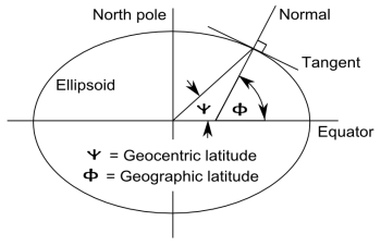
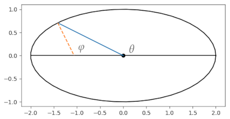
From a given point on the earth’s surface, draw two lines: one straight down (i.e. perpendicular to the surface) and one straight to the center of the earth. The angle φ that the former makes with the equatorial plane is geographic latitude. The angle θ that the latter makes with the equatorial plane is geocentric latitude.

For illustration we will draw an ellipse that is far more eccentric than a polar cross-section of the earth.

At first it may not be clear why geographic latitude is defined the way it is; geocentric latitude is conceptually simpler. But geographic latitude is easier to measure: a plumb bob will show you which direction is straight down.

There may be some slight variation between the direction of a plumb bob and a perpendicular to the earth’s surface due to variations in surface gravity. However, the deviations due to gravity are a couple orders of magnitude smaller than the differences between geographic and geocentric latitude.

Conversion formulas

The conversion between the two latitudes is as follows.

$\begin{align*} \theta &= \text{atan2}((1 - e^2)\sin\varphi, \cos\varphi) \\ \varphi &= \text{atan2}(\sin\theta, (1 - e^2)\cos\theta) \end{align*}$

Here e is eccentricity. The equations above work for any ellipsoid, but for earth in particular e² = 0.00669438.

The function atan2(y, x) returns an angle in the same quadrant as the point (x, y) whose tangent is y/x. [1]

As a quick sanity check on the equations, note that when eccentricity e is zero, i.e. in the case of a circle, φ = θ. Also, if φ = 0 then θ = φ for all eccentricity values.

Next we give a proof of the equations above.

Proof

We can parameterize an ellipse with semi-major axis a and semi-minor axis b by

$(x(t), y(t)) = (a \cos t, b \sin t)$

The slope at a point (x(t), y(t)) is the ratio

$\frac{y^\prime(t)}{x^\prime(t)} = \frac{b \cos t}{-a \sin t}$

and so the slope of a line perpendicular to the tangent, i.e tan φ, is

$\tan \varphi = \frac{a \sin t}{b \cos t} = \frac{a}{b} \tan t$

Now

$\tan \theta = \frac{b \sin t}{a \cos t} = \frac{b}{a} \tan t$

and so

$\begin{align*} \tan \varphi &= \frac{a}{b} \tan t \\ &= \frac{a}{b} \left( \frac{a}{b} \tan \theta \right) \\ &= \frac{a^2}{b^2} \tan \theta \\ &= \frac{1}{1 - e^2} \tan \theta \end{align*}$

where e² = 1 − b²/a² is the eccentricity of the ellipse. Therefore

$(1 - e^2) \tan \varphi = \tan \theta$

and the equations at the top of the post follow.

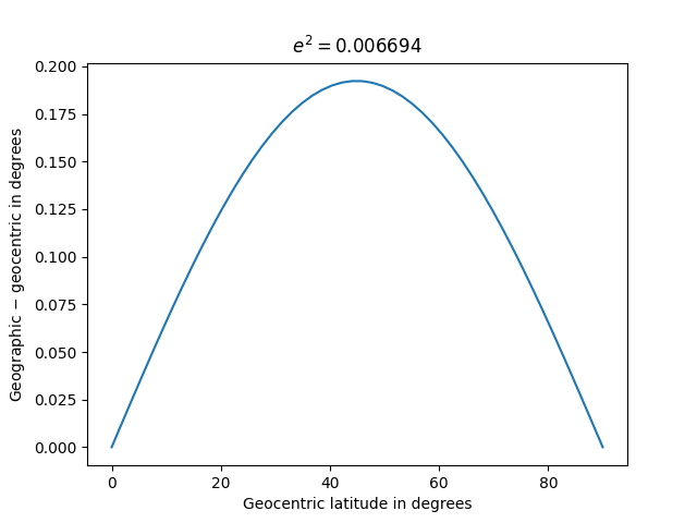
Difference

For the earth’s shape, e² = 0.006694 per WGS84. For small eccentricities, the difference between geographic and geocentric latitude is approximately symmetric around 45°.

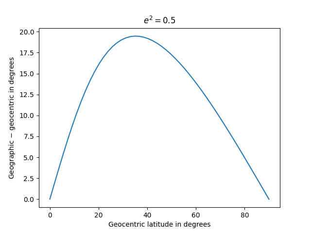
But for larger values of eccentricity the asymmetry becomes more pronounced.

[1] There are a couple complications with programming language implementations of atan2. Some call the function arctan2 and some reverse the order of the arguments. More on that here.

Mason, Dixon, and Latitude

Posted on 23 December 2025 by John

A few weeks ago I mentioned that I was reading Stephen Ambrose’s account of the Lewis & Clark expedition and wrote a post about their astronomical measurements. James Campbell left a comment recommending Edwin Danson’s book [1] on the history of the Mason-Dixon line. I ordered the book, and now that work has slowed down for Christmas I have had the time to open it.

In addition to determining their eponymous line, surveyors Charles Mason and Jeremiah Dixon were also the first to measure a degree of latitude in 1767.

Observations for determining the Length of a Degree of Latitude in the Provinces of Maryland and Pennsylvania, in North America, by Messieurs Charles Mason and Jeremiah Dixon

What exactly did they measure? We’ll get to that, but first we need some background.

The shape of the Earth

To first approximation a degree of latitude is simply 1/360th of the Earth’s circumference, but Mason and Dixon were more accurate than that. Isaac Newton (1643–1727) deduced that our planet was not a perfect sphere but rather an oblate spheroid. The best measurement in Mason and Dixon’s time was that the Earth’s semi-major axis was 6,397,300 meters with flattening 1/f = 216.8.

It’s a bit of an anachronism to describe the distance in meters since the meter was defined in 1791. The meter was originally defined as one ten-millionth of the distance from the equator to the North Pole along a great circle through Paris.

What exactly is a degree of latitude?

If the Earth were a perfect sphere, a degree of latitude would be 1/360th of its circumference. Using the original definition of the meter, this would be exactly 10,000,000/360 meters. But because the Earth is not a perfect sphere, each degree of latitude has a slightly different length. To put it another way, the length of a degree of latitude varies by latitude.

Another complication due to the flattening of the Earth is that there are multiple ways to define latitude. The two most common are geocentric and geodetic. The geocentric latitude of a point P on the Earth’s surface is the angle between the equatorial plane and a line between the center of the earth and P. The geodetic latitude (a.k.a. geographic latitude) of P is the angle between the equatorial plane and a line perpendicular to the Earth’s surface at P. More on the difference between geocentric and geodetic latitude here.

What did Mason and Dixon measure?

Since the length of a degree of latitude varies, we need to say at what latitude they measured the length of a degree. In short, they measured the length of a degree near what we now know as the Mason-Dixon line, the border between Pennsylvania and Maryland.

To be more precise, the starting point was Stargazer’s Stone, a stone placed by Mason and Dixon on John Harland’s farm near Embreeville, Pennsylvania, to a point about a degree and a half due south near what is now Delmar, a town on the Delaware / Maryland border.

I’ve had some difficulty determining how accurate Mason and Dixon were. Some sources I’ve found are obviously wrong. I haven’t verified this, but it seems Mason and Dixon overestimated the length of a degree of latitude at their location by only 465.55 ft or about 0.13%, a remarkable feat given the technology of their day.

[1] Edwin Danson. Drawing The Line: How Mason and Dixon Surveyed the Most Famous Border in America. John Wiley & Sons. 2001.

Spherical coordinate Rosetta Stone

Posted on 12 August 2023 by John

If you’ve only seen one definition of spherical coordinates, you may be shocked to discover that there are multiple conventions. In particular, mathematicians and geoscientists have different conventions. As Volker Michel put it in book on constructive approximation,

Many mathematicians have faced weird jigsaw puzzles with misplaced continents after using a data set from a geoscientist.

Nor are there only two conventions. This post will cover three conventions, which I will call physics, math, and geography. This is not to imply that everyone in a profession uses the conventions named after the profession.

As with Fourier transforms there are many conventions. Presumably the reason for the proliferation of conventions is the same: a useful basic concept will be discovered multiple times in different areas of application. When there are trade-offs between conventions, people working in each area will choose the convention that is simplest for the things they care most about.

Questions and definitions

Given a triple of numbers (c₁, c₂, c₃), that represent spherical coordinates, there are two basic questions:

What do the numbers mean?
What symbol should be used to represent them?

Part of the meaning question is whether the coordinate system is left-handed or right-handed. There is also a minor question of the standard range of equivalent angles.

Polar angle is the angle down from the positive z-axis, the north pole. The north pole has polar angle 0 and the south pole has polar angle π.

Latitude is the angle up from the xy plane or the equator. The latitude of the north pole is π/2 and the latitude of the south pole is −π/2.

Azimuth is the angle from an initial meridian (e.g. the Prime Meridian in geography). In mathematical terms it is the angle between the x-axis and a line connecting the projection of a point to the xy to the origin.

Physics convention

The physics convention is also the ISO 80000-2 convention. The three coordinates are

(radial distance to origin, polar angle, azimuthal angle)

and are conventionally denoted

(r, θ, ϕ).

The point (r, θ, ϕ) corresponds to

(r sin θ cos ϕ, r sin θ sin ϕ, r cos θ)

in Cartesian coordinates.

The coordinate system is right-handed: ϕ increases in the counterclockwise direction when looking down on the xy plane.

The polar angle typically runs from 0 to π and the azimuthal angle typically runs from 0 to 2π.

Math convention

In this convention the three coordinates are

(radial distance to origin, azimuthal angle, polar angle)

and are denoted

(ρ, θ, ϕ).

When compared to the physics notation we have something of a Greek letter paradox. Both conventions agree that the second coordinate should be written θ and the third coordinate should be written ϕ, but the two conventions mean opposite things by the two symbols.

The advantage of using θ to denote the azimuthal angle is that then θ has the same meaning as it has in polar coordinates. Similarly, the advantage of using ρ rather than r is to preserve the meaning of r in polar and cylindrical coordinates: ρ is the distance in 3 dimensions from a point to the origin, and r is the distance in 2 dimensions from the projection of a point to the xy plane and the origin.

Sometimes you’ll see r rather than ρ for the first coordinate.

The point (ρ, θ, ϕ) corresponds to

(ρ cos θ sin ϕ, ρ sin θ sin ϕ, ρ cos ϕ).

The math convention uses the same orientation and typical range coordinate ranges as the physics convention.

Geography and geoscience

Geographic coordinate systems are complicated by the fact that the earth is not perfectly spherical. Geographic latitude and geocentric latitude are not exactly the same as the following highly exaggerated diagram shows.

However, for this post we will assume a perfectly spherical earth in which geographic and geocentric latitudes are the same.

A point on the earth’s surface is described by two numbers, latitude and longitude. This corresponds to spherical coordinates in which the first coordinate is implicitly the earth’s radius. You’ll see latitude and longitude listed in either order.

The polar angle is sometimes called colatitude because latitude is the complementary angle of latitude. Longitude corresponds to azimuth. There are multiple symbols used for latitude, though λ is common for longitude. If you see one coordinate denoted λ, the other is latitude.

The safest, most explicit notation is to use the words longitude and latitude, not depending on symbols or order. Longitude is implicitly longitude east of the Prime Meridian, but to be absolutely clear, put an E at the end. Latitude typically ranges from −π/2 to π/2 (−90° to 90°). Longitude either runs from 0 to 2π or from −π to π (−180° to 180°).

To convert to Cartesian coordinates, set polar angle to π/2 − latitude, azimuth to longitude (east), and use the formulas above for either the physics or mathematics notation. If you have elevation, this is the radial distance above the earth’s surface, so ρ is the earth’s radius plus elevation.

How faithful can a map be?

Posted on 10 May 2023 by John

It’s well known that you cannot map a sphere onto the plane without distortion. You can’t map the entire sphere to the plane at all because a sphere and a plane are not topologically equivalent.

But even if you want to map a relatively small portion of globe to paper, say France, with about 0.1% of the globe’s area, you’ll have to live with some distortion. How can we quantify this distortion? How small can it be?

We know the result has to vary with area. We expect it to approach zero as area on the globe goes to zero: the world is not flat, but it is locally flat. And we expect the amount of distortion to go to infinity as we take in more of the globe’s area. We expect to be able to make a map of France without too much distortion, less distortion than making a map of Australia, but more distortion than making a map of Lichtenstein.

This problem was solved a long time ago, and John Milnor wrote an expository article about it in 1969 [1].

Defining distortion

The way to quantify map distortion is to look at the ratio of distances on the globe to distances on paper. We measure the distance between points on the globe by geodesic distance, the length of the shortest path between two points. We’d like the ratio of distances on a globe to distances on a map to be constant, but this isn’t possible. So we look at the minimum and maximum of this ratio. In a good map these two ratios are roughly the same.

Milnor uses

d_S(x, y)

to denote the distance between two points x and y on a sphere, and

d_E(f(x), f(y))

for the distance between their image under a projection to the Euclidean plane.

The scale of a map with respect to points x and y is the ratio

d_E(f(x), f(y)) / d_S(x, y).

Let σ₁ be the minimum scale as x and y vary and let σ₂ be the maximum scale. The distortion of the projection f is defined to be

δ = log(σ₂/σ₁).

When σ₁ and σ₂ are approximately equal, δ is near 0.

Example: Mercator projection

One feature of the Mercator projection is that there is no distortion along lines of constant latitude. Given two points on the equator (less than 180° apart) their distance on a Mercator projection map is strictly proportional to their distance on the globe. The same is true for two points on the flat part of the US-Canada border along the 49th parallel, or two points along the 38th parallel dividing North Korea and South Korea.

For points along a parallel (i.e. a line of latitude) the scale is constant, such as a thousand miles on the globe corresponding to an inch on the map. We have σ₁ = σ₂ and so δ = 0.

The distortion in the Mercator projection is all in the vertical direction; distances along a meridian are distorted. Mercator maps latitude φ to something proportional to

φ ↦ log( sec φ + tan φ ).

Near the equator sec φ ≈ 1, tan φ ≈ φ, and the image of φ is approximately φ. But as φ approaches 90° the secant and tangent terms become unbounded and the distortion goes to infinity. You could use the equation for the Mercator projection of latitude to calculate the distortion of a “rectangle on a globe.”

Minimizing distortion

Let D_α be a disk geodesic radius α radians where 0 < α < π. Then Milnor shows that the minimum possible distortion when mapping D_α to the plane is

δ₀ = log(α / sin α).

This map is realizable, and is unique up to similarity transformations of the plane. It is known in cartography as the azimuthal equidistant projection.

For small values of α the distortion is approximately α²/6, or 2/3 of the ratio of the area of D_α to the area of the globe.

We said earlier that France takes up about 0.1% of the earth’s surface, and so the minimum distortion for a map of France would be on the order of 0.0007.

[1] John Milnor. A Problem in Cartography. American Mathematical Monthly, December 1969, pp. 1102–1112.

Area of a “rectangle” on a globe

Posted on 21 February 2023 by John

What do we mean by rectangle?

This post will derive the area of a spherical region bounded by lines of latitude and longitude. Such a region corresponds to an actual rectangle on a Mercator projection map, with sides aligned with the coordinate axes, and is approximately a rectangle on a sphere if the rectangle is not too big [1].

What do we know up front?

Before we get into detailed equations, we know that the area will be proportional to the difference in longitude. If we’re looking that the area between two parallels, such as the equator and the Arctic Circle, the area between 10° and 20° longitude is the same as the area between 80° and 90° longitude, and twice the area between 72° and 77° longitude.

The difficulty is latitude. Say we look at squares on a map that are 1° of longitude wide and 1° of latitude tall. Those squares are on the map will correspond to more area on the globe for latitudes near the equator, and less area at high latitudes.

So the area bounded by longitudes θ₁ and θ₂ and latitudes φ₁ and φ₂ will depend on φ₁ and φ₂ individually, but only on the difference θ₁ − θ₂.

Spherical caps

The region on a sphere above a fixed line of latitude is called a spherical cap. The northern hemisphere, the region above the equator, would be a very large spherical cap. The region inside the Arctic Circle would be a smaller spherical cap.

Let R be the radius of the earth. Then the surface area above a latitude φ is

A = 2πR²(1 − sin φ).

You could derive this using calculus by thinking of the spherical cap as a surface of revolution.

Spherical bands

Given two latitudes φ₁ and φ₂ with latitudes φ₁ > φ₂, the area of a band between latitude φ₁ and latitude φ₂ is the area of the spherical cap above latitudes φ₂ minus the area of the spherical cap above latitudes φ₁. This gives

A = 2πR²(sin φ₁ − sin φ₂).

Area of latitude/longitude grid

Now we can find the area of the region bounded by longitudes θ₁ and θ₂ and latitudes φ₁ and φ₂. The total area between latitudes φ₁ and φ₂ is given by the equation above. The subset of this area between longitudes θ₁ and θ₂ is proportional to θ₁ − θ₂. If longitude is measured in radians then

A = R² (sin φ₁ − sin φ₂) (θ₁ − θ₂).

If longitude is measured in degrees, we have

A = π R² (sin φ₁ − sin φ₂) (θ₁ − θ₂)/180.

[1] As Nathan helpfully pointed out in the comments, it might be clearer to say “not too big and not too close to one of the poles.” Another way to put it might be to say the idea of what is “big” depends on how close to a pole you are.

Law of cosines on a sphere

Posted on 24 August 2022 by John

The previous post looked at the analog of the Pythagorean theorem on a sphere. This post looks at the law of cosines on a sphere.

Yesterday we looked at triangles on a sphere with sides a and b meeting at a right angle and hypotenuse c. Denote the angle opposite a side with the capital version of the same letter, so C is the angle opposite c. We assumed C is a right angle, but now we will remove that assumption.

The spherical analog of the law of cosines says

cos(c) = cos(a) cos(b) + sin(a) sin(b) cos(C).

Note that we have two kinds of angles: the arcs that make up the sides, and the angle formed by the intersection of arcs [1]. So the cos(C) term at the end is different animal from the other terms in the equation.

If C is a right angle, cos(C) = 0 and the second term drops out, leaving us with the spherical counterpart of the Pythagorean theorem. But we do not require that C be a right angle.

Application to air distance

Suppose we want to find how far a plane would travel between Los Angeles (LAX) and Houston (IAH), assuming it takes a great circle path. The lat/long coordinates of the two airports are (33.94°, −118.41°) and (29.98°, −95.34°).

Los Angeles and Houston are approximately at the same latitude, but even if they were at exactly the same latitude we couldn’t just find the flight distance by finding the length of the arc of constant latitude between them because that arc would not be part of a great circle.

To find the distance between LAX and IAH we form a triangle with vertices at LAX, IAH, and the north pole. Call the arc from LAX to the north pole a and the arc from IAH to the north pole b. Since latitude is the angle up from the equator, the angle down from the pole is 90° minus latitude. So

a = 90° − 33.94° = 56.06°

and

b = 90° − 29.98° = 60.02°

The arcs a and b meet at the angle C equal to the differences in the two longitudes. That is,

C = 118.41° − 95.34° = 23.07°.

The law of cosines

cos(c) = cos(a) cos(b) + sin(a) sin(b) cos(C)

reduces to

cos(c) = cos(56.06°) cos(60.02°) + sin(56.06°) sin(60.02°) cos(23.07°)

in our problem.

This tells us

cos(c) = 0.9402

from which we find c = 0.3477 radians or 19.92°. Assume the earth is a perfect sphere of radius r = 3959 miles. The arc length we’re after is r times c in radians, or 1376 miles.

[1] In the language of differential geometry, the arcs are geodesics on the sphere and the angles of intersection are measured in the tangent space at the intersection point.

Pythagoras on a sphere

Posted on 23 August 2022 by John

Suppose you drive a distance a, turn right, then drive a distance b. How far are you from where you started?

If a and b are relatively small, then the answer is given by the Pythagorean theorem. Small here means small relative to the radius of the Earth. Any distance you drive is small enough: it matters more that roads are not perfectly straight than that the Earth is not perfectly flat.

Now suppose you fly a distance a, turn right, then fly a distance b. Now how far are you from where you started? Now the curvature of the earth might matter a good deal, and the Pythagorean theorem could give you a poor answer.

Spherical version of the Pythagorean theorem

If a and b are moderately large, we need to look at spherical triangles, not plane triangles. A “straight” line on a sphere is a piece of a great circle, a circle whose center is the center of the sphere. A spherical triangle has three straight sides, straight in the sense of a straight line on a sphere. We need to consider a spherical triangle with sides a and b that meet at right angles, and we want to find the length of the hypotenuse c of the spherical triangle.

The spherical analog of the Pythagorean theorem says

cos(c) = cos(a) cos(b).

This looks weird the first time you see it, because you’re taking the cosine of a side rather than an angle. But on a sphere, the sides are angles. For example, if a side of the triangle is on a meridian, we could measure its length in degrees of latitude. But the theorem above does not require sides to be lined up with any coordinate system. It only requires that the sides a and b meet at a right angle.

Small spherical triangles

Let’s suppose for a moment that a and b are small when measured in radians, small enough that a², b², and ab are negligible compared to a and b. Then we can use the approximation

cos(x) ≈ 1 − x²/2

in the theorem above to show that

c² ≈ a² + b².

This is reassuring since we know the Pythagorean theorem holds for human-scale distances on our planet.

Example with a big triangle

Quito to Nairobi to Jerusalem and back to Quito

Now let’s look at a big triangle. The vertices have longitude and latitude (−80°, 0°), (35°, 0°), and (35°, 30°). These correspond approximately to Quito, Nairobi, and Jerusalem. So a = 115° and b = 30°. We can solve for c and find it equals 111°.

A minute of latitude is a nautical mile; the nautical mile is defined the way to make these kinds of calculations easier. A nautical mile is about 15% longer than a mile.

A degree of a great circle is 60 nautical miles. So our hypotenuse of 111 degrees is 6,660 nautical miles. If we had used the Pythagorean theorem, we would have overestimated this distance as 7,130 nautical miles.

Notice that the triangle with vertices at Quito, Nairobi, and Jerusalem doesn’t look like a triangle when projected flat. Two legs look straight because they follow lines of constant latitude or longitude. But the flight from Jerusalem to Quito is just as straight as the other flights if you look at it on a globe.

Not so great circles

In the example above, I chose Quito and Nairobi because they were near the equator. The equator is a great circle.

Suppose I’d chosen Houston and Wuhan instead. Both cities are at about 30° latitude. I could not find the distance between the two cities by simply subtracting their longitudes because the 30th parallel is not a great circle. Spherical geometry is generally more involved than in the example above.

A great circle path from Houston to Wuhan would not follow the 30th parallel but would actually cross Alaska. The great circle distance is 6,800 nautical miles. Flying along a path of 30° latitude would add an extra 1,000 nautical miles to the flight.

A tale of three cities

Posted on 26 November 2021 by John

Big blue marble

Pick three cities and form a spherical triangle by connecting each pair of cities with the shortest arc between them. How might you find the area of this triangle?

For this post, I’ll assume the earth is perfectly spherical. (Taking into account that the earth is slightly oblate makes the problem much more complicated. Maybe a post for another time.)

Spherical excess

If you draw a triangle on the plane, the interior angles add up to 180°. But if you draw a triangle on a sphere, the interior angles add up to more than 180°. The amount by which the sum of the interior angles exceeds 180° is called the spherical excess. It turns out that the area of a spherical triangle is proportional to its spherical excess.

For example, if a spherical triangle is small relative to the radius of the sphere, it’s nearly a Euclidean triangle, and the spherical excess is negligible. But consider a much bigger spherical triangle, one with a vertex at the north pole and vertices at two points 90° apart on the equator. This triangle has three right angles, so the sum of the interior angles is 270° and the spherical excess is 90°.

Relating spherical excess and area

If we measure spherical excess E in radians, then the area of a spherical triangle is

A = ER²

where R is the radius of the sphere. This remarkable theorem was discovered by Thomas Harriot in 1603.

Let’s go back to the example above of a triangle running from the north pole to two points 90° apart on the equator. This triangle takes up 1/8 of the earth’s surface, and area of the earth is 4πR², and so the triangle has area πR²/2. In this case the spherical excess E was π/2, and so we could have come to the same result by multiplying E by R².

Computing area

We can find the area of a spherical triangle by measuring the angle of arcs between pairs of points. We’ll compute area assuming the sphere has radius 1. (Otherwise temporarily assume radius 1 and then multiply by R² when we’re done.)

The previous post explains how to find a parameterization for the great circle connecting points on a sphere. We can take derivatives to find tangent vectors where the great circles intersect, and compute the angle between these tangents to find the interior angles of our triangles.

The previous post showed that if the central angle between two vectors A and B is θ then

cos(t) A + sin(t) (cot θ A – csc θ B)

parameterizes a great circle including A and B. This curve passes through A at time t = 0 with velocity

cot θ A – csc θ B

and so this gives us a tangent vector at A in the direction of B. Repeat the exercise for a great circle between A and C. Then the cosine of the angle of intersection is the two normalized tangent vectors. We can thus obtain all the interior angles, and from there we can compute the spherical excess and thus the area of the spherical triangle.

Maidenhead geocode system

Posted on 30 May 2021 by John

The Maidenhead Locator System encodes a pair of longitude and latitude coordinates in a slightly complicated but ingenious way. Amateur radio operators using this geocoding system to describe locations.

The Wikipedia article on the subject describes the what of the system, but I’d like to say more about the why of the system. I’ll also go through an example in great detail. Continue reading →

Spherical trig, Research Triangle, and Mathematica

Posted on 3 December 2018 by John

This post will look at the triangle behind North Carolina’s Research Triangle using Mathematica’s geographic functions.

Spherical triangles

A spherical triangle is a triangle drawn on the surface of a sphere. It has three vertices, given by points on the sphere, and three sides. The sides of the triangle are portions of great circles running between two vertices. A great circle is a circle of maximum radius, a circle with the same center as the sphere.

An interesting aspect of spherical geometry is that both the sides and angles of a spherical triangle are angles. Because the sides of a spherical triangle are arcs, they have angular measure, the angle formed by connecting each vertex to the center of the sphere. The arc length of a side is its angular measure times the radius of the sphere.

Denote the three vertices by A, B, and C. Denote the side opposite A by a, etc. Denote the angles at A, B, and C by α, β, and γ respectively.

Research Triangle

Research Triangle is a (spherical!) triangle with vertices formed by Duke University, North Carolina State University, and University of North Carolina at Chapel Hill.

(That was the origin of the name, though it’s now applied more loosely to the general area around these three universities.)

We’ll take as our vertices

A = UNC Chapel Hill (35.9046 N, 79.0468 W)
B = Duke University in Durham (36.0011 N, 78.9389 W),
C = NCSU in Raleigh (35.7872 N, 78.6705 W)

Research Triangle

Mathematica

We’ll illustrate several features of Mathematica using the spherical triangle corresponding to Research Triangle.

Map

The map above was produced with the following Mathematica code.

    ptA = GeoPosition[{35.9046, -79.0468}]
    ptB = GeoPosition[{36.0011, -78.9389}]
    ptC = GeoPosition[{35.7872, -78.6705}]

    GeoGraphics[{Red, PointSize[Large], 
        Point[ptA], Point[ptB], Point[ptC]}, 
        GeoScaleBar -> "Imperial", 
        GeoRange -> 29000]

Note that longitude is in degrees east, so the longitudes above are negative.

Distance

To find the distance between two locations, you can use the function GeoDistance. For example,

    GeoDistance[ptA, ptB]

tells me that the distance between UNC and Duke is 8.99185 miles. I assume it displays miles by default based on my location in the US, though the GeoRange option above defaults to meters. You can make the system of units explicit. For example

    GeoDistance[ptA, ptB, UnitSystem -> "Metric"]

returns 14.741 km.

If we want to find the length of the side c in degrees, we can use the Earth’s radius.

    r = PlanetData["Earth", "Radius"]
    c = GeoDistance[ptA, ptB] 360 / (2 Pi r)

This shows that c is 0.13014°. Calculating the other sides similarly shows a = 0.30504° and b = 0.32739°.

Angles

Calling GeoDirection[ptA, ptB] returns 42.2432°, which says we need to head at an angle of about 42° to walk from UNC to Duke.

The code

    GeoDirection[ptA, ptB] - GeoDirection[ptA, ptC]

shows that the angle α is 68.6128°. (The code returns the negative of this angle because the angle is clockwise.) Similarly we find β = 87.9808° and γ = 23.4068.

The angles add up to 180° only because our triangle is small compared to the earth’s total area. The actual sum should be slightly more than 180°, but we’ve not retained enough precision to detect the difference. In general the “spherical excess,” i.e. the amount by which the sum of the angles exceed 180°, is proportional to the area of the triangle.

Conversion formulas

Proof

Difference

Related posts

The shape of the Earth

What exactly is a degree of latitude?

What did Mason and Dixon measure?

Related posts

Questions and definitions

Physics convention

Math convention

Geography and geoscience

Related posts

Defining distortion

Example: Mercator projection

Minimizing distortion

What do we mean by rectangle?

What do we know up front?

Spherical caps

Spherical bands

Area of latitude/longitude grid

Related posts

Application to air distance

Related posts

Spherical version of the Pythagorean theorem

Small spherical triangles

Example with a big triangle

Not so great circles

Related posts

Spherical excess

Relating spherical excess and area

Computing area

Related posts

Spherical triangles

Research Triangle

Mathematica

Map

Distance

Angles

More spherical trig posts